Linear Approximation calculator

This linearization calculator will allow to compute the linear approximation, also known as tangent line for any given valid function, at a given valid point.

You need to provide a valid function like for example f(x) = x*sin(x), or f(x) = x^2 - 2x + 1, or any valid function that is differentiable, and a point \(x_0\) where the function is well defined. This point can be any valid numeric expression, like 1/3, for example.

Once you provide a valid function and point, you click on "Calculate" and all the calculations will be shown for you.

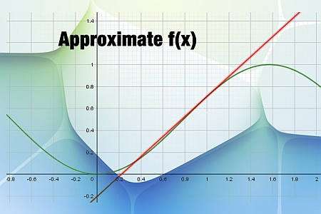
Linear or first order approximation look for an approximation of the given function by a line, at a given point \(x_0\). Naturally for curves a linear approximation will be rough, though the main idea is that the approximation will be accurate for points close to \(x_0\).

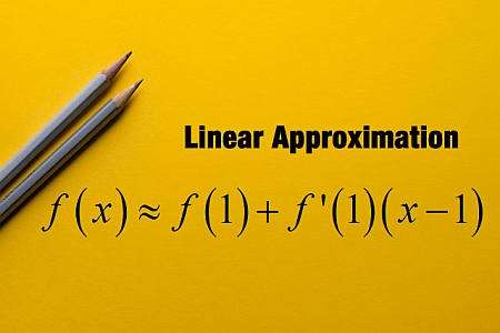
Linear Approximation

The idea is to find a line that passes through the point \((x_0, f(x_0))\) and it "barely touches" the function \(f(x)\). The formal mathematical definition of 'barely touching' is given by the idea of tangent line, for which we need to compute the derivative of the function.

In fact, the formula for the linear approximation at the point \(x_0\) depends on the derivative \(f'(x_0)\), as follows

\[\displaystyle y = f(x_0) + f'(x_0) (x - x_0) \]

This linear approximation formula essentially defines the equation of a line that passes through the point \((x_0, f(x_0))\), which is why is called "linear approximation", since it defines a linear function that coincides with \(f(x)\) at the point \(x_0\), and it is very close to \(f(x)\) for values of \(x\) that are close to \(x_0\).

Steps for finding the linear approximation

• Step 1: You need to have a given function f(x) and a point x0. The function must be differentiable at x0
• Step 2: Compute f(x0) and f'(x0), which are the function and derivative of the function f at the point x0
• Step 3: Define the linear approximation as y = f(x_0) + f'(x_0) (x - x_0), which is the linearization formula presented above

This line, \(y = f(x_0) + f'(x_0) (x - x_0)\) represents the first order approximation, also known as local linear approximation.

Link with tangent line

As you have probably suspected by now, the linear approximation is the same as the tangent line at the given point. Then, calculating the linear approximation is exactly the same as calculating the tangent line

Another name for the same is first order approximation, or tangent line approximation, which are commonly used names in Calculus as well.

Differential and Linear approximation

Another common concept is that of differential, which is tightly linked to that of the linear approximation, and it is simply a derivation of it. Indeed, the differential (or finite difference) is defined as \(\Delta y = y - f(x_0)\). So then, based on the first order approximation formula, the formula for the differential is

\[\displaystyle \Delta y = y - f(x_0) = f'(x_0) (x - x_0) = f'(x_0) \Delta x \]

This naturally looks exactly like the linear approximation formula, except that the term \(f(x_0\) is passed to the left.

Example: Calculating of first order approximation.

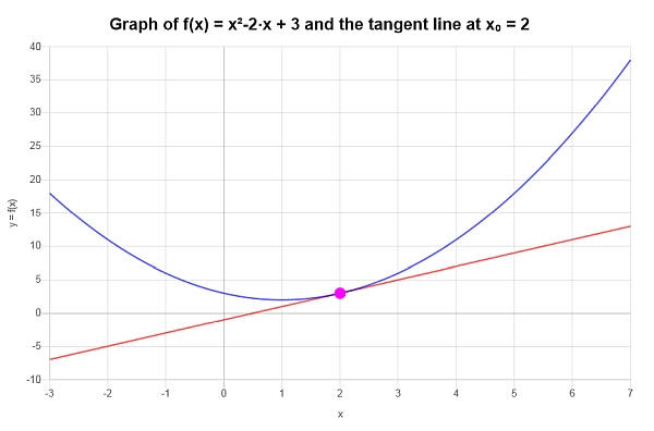
Consider the following: \(f(x) = x^2 - 2x + 3\), find its first order approximation at \(x_0 = 1\).

Solution: The function that has been provided is \(\displaystyle f(x)=x^2-2x+3\), and we need to find the linear approximation around the point x = 1. So then, we first need the derivative.

Linear Approximation: The equation for the linear approximation that we are looking for at the point \(x_0 = 2\) is given by the following formula

\[y = y_0 + f'(x_0)(x - x_0) \]

Notice that by definition \(\displaystyle y_0 = f(x_0)\), which implies that we need to plug the function at the point \(x_0 = 2\) :

\[y_0 = f(x_0) = f\left(2\right) = 2^2-2\cdot 2+3 = 3\]

We do the same, but now for the derivative at the point \(x_0 = 2\), so then

\[f'(x_0) = f'\left(2\right) = 2\cdot 2-2 = 2 \]

Now with this, we come back to the linear approximation formula:

\[y = y_0 + f'(x_0)(x - x_0) \]\[\Rightarrow y = 3+2\left(x-2\right) = 2x-1 \]

Conclusion: We conclude that the linear approximation for \(\displaystyle f(x)=x^2-2x+3\) at \(x_0 = 2\) is given by:

\[y = 2x-1 \]

Graphically:

Example: More first order approximation

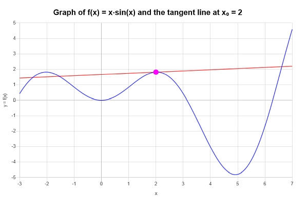
For the function : \(f(x) = x \sin(x)\) and the point \(x_0 = 2\), find the corresponding first order approximation.

Solution:In this case, the function we need to work is: \(\displaystyle f(x)=x\sin\left(x\right)\).

We now calculate its derivative:

Linear Approximation: The equation of the linear approximation is:

\[y = y_0 + f'(x_0)(x - x_0) \]

where \(\displaystyle y_0 = f(x_0)\), so then we compute:

\[y_0 = f(x_0) = f\left(2\right) = 2\sin\left(2\right)\]

For the derivative at \(x_0 = 2\) we find that:

\[f'(x_0) = f'\left(2\right) = 2\cos\left(2\right)+\sin\left(2\right) \]

Now we are ready to put these back into the the first order approximation formula:

\[y = y_0 + f'(x_0)(x - x_0) \]\[\Rightarrow y = 2\sin\left(2\right)+2\cos\left(2\right)+\sin\left(2\right)\left(x-2\right) = 2x\cos\left(2\right)+x\sin\left(2\right)-4\cos\left(2\right) \]

Conclusion: It is concluded that the linear approximation of \(\displaystyle f(x)=x\sin\left(x\right)\) at the given point \(x_0 = 2\) is computed as:

\[y = 2x\cos\left(2\right)+x\sin\left(2\right)-4\cos\left(2\right) \]

Graphically, we get the following plot:

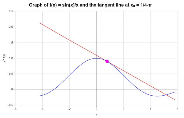
Example: Linear Approximation calculation

Calculate the first order approximation for \( f(x) = \frac{\sin(x)}{x}\) at \(x = \frac{\pi}{4}\).

Solution:The following function has been provided: \(\displaystyle f(x)=\frac{\sin\left(x\right)}{x}\), for which we need to compute its derivative.

The function came already simplified, so we can proceed directly to compute its derivative:

First Order Approximation: The equation for the corresponding first order approximation for the given function \(\displaystyle f(x)=\frac{\sin\left(x\right)}{x}\) at the given point \(x_0 = \frac{\pi}{4}\) is given by the following:

\[y = y_0 + f'(x_0)(x - x_0) \]

Plugging the corresponding values:

\[y_0 = f(x_0) = f\left(\frac{\pi}{4}\right) = \frac{\sin\left(\frac{\pi{}}{4}\right)}{\frac{\pi{}}{4}} = \frac{2\sqrt{2}}{\pi{}}\] \[f'(x_0) = f'\left(\frac{\pi}{4}\right) = \frac{\cos\left(\frac{\pi{}}{4}\right)}{\frac{\pi{}}{4}}-\frac{\sin\left(\frac{\pi{}}{4}\right)}{\left(\frac{\pi{}}{4}\right)^2} = \frac{2\sqrt{2}}{\pi{}}-\frac{8\sqrt{2}}{\pi{}^2} \]

So now we can put this in the formula:

\[y = y_0 + f'(x_0)(x - x_0) \] \[\Rightarrow y = \frac{2\sqrt{2}}{\pi{}}+\frac{2\sqrt{2}}{\pi{}}-\frac{8\sqrt{2}}{\pi{}^2}\left(x-\frac{1}{4}\pi{}\right) = -\frac{1}{2}\sqrt{2}+\frac{2\sqrt{2}x}{\pi{}}+\frac{4\sqrt{2}}{\pi{}}-\frac{8\sqrt{2}x}{\pi{}^2} \]

Conclusion: We can conclude therefore that the first order approximation for the given function \(\displaystyle f(x)=\frac{\sin\left(x\right)}{x}\) at the given point \(x_0 = \frac{\pi}{4}\) is given by

\[y = -\frac{1}{2}\sqrt{2}+\frac{2\sqrt{2}x}{\pi{}}+\frac{4\sqrt{2}}{\pi{}}-\frac{8\sqrt{2}x}{\pi{}^2} \]

The following is obtained graphically:

More derivatives calculators

Aside from this linearization calculator, you can find a lot that do different things based on derivatives. Differentiation is a crucial operation in Calculus, Physics, Engineering and Economics, with a broad spectrum of applications.

There is also a way to conduct a linear approximation for more variables, this is for example, for a function \f(x, y)\), in which case the linear approximation formula becomes \(f(x, y) = f(x_0, y_0) + \frac{\partial f}{\partial x}(x_0, y_0)(x-x_0) + \frac{\partial f}{\partial y}(x_0, y_0)(y-y_0)\), so then in this case, in order to find the linearization we need to use partial derivatives.

Finding the linearization of a function is not by far the only thing you can do with derivatives. Differentiation is a relatively easy operation with simple rules like the product rule, the quotient rule and the chain rule that makes the calculation of derivatives a relatively straightforward operation.

Although it is supposed to be simple, it is a good idea to use a derivative calculator to get all the steps shown, with a clear mention of all the derivative rules used.