Computing Price Elasticity of Demand from Sample Data

Use this calculator to estimate the price elasticity of demand based on sample data for price and quantity demanded that you provide.

You will need to provide valid sample data, in terms of both samples (price and quantity demanded) being positive values. Once you have your data pasted in the spreadsheet, you can click on "Calculate" to get all the steps shown.

Observe that this approach requires the data to follow a specific pattern that suits a log-log model, where \(\ln(P)\) and \(\ln(Q)\) are used as auxiliary variables to conduct a linear regression model.

Calculating Price Elasticity from Sample Data

In order to compute the price elasticity, you will need to estimate the following auxiliary model:

\[\displaystyle \ln(Q) = a + b \ln(P) \]

Notice that this corresponds to a regular linear regression model with he original variables price and quantity being log-transformed. That is why we require both variables to be strictly positive.

What are the steps for calculating the elasticity?

• Step 1: Identify the sample data for the variables provided for price (P) and quantity (Q)
• Step 2: Make sure both samples have the sample sample size and that they are BOTH positive, otherwise you won't be able to do the calculation
• Step 3: Log-transform both variables: Compute ln(X) and ln(Y)
• Step 4: Conduct an auxiliary linear regression for the variables ln(X) and ln(Y), where ln(X) is the independent variable and ln(Y) is the dependent variable
• Step 5: The slope coefficient found for this auxiliary regression is the price elasticity of demand for these data

The crucial step then is the log-transformation of the data, which allows us to compute the elasticity based on the results of a linear regression, making the results found highly interpretable.

Understanding Price Elasticity

By definition, price elasticity is defined by using the following formula:

\[ \varepsilon = \displaystyle \frac{\% \Delta Q }{\% \Delta P} \]

This indicates that, among other things, we can predict the percent change of quantity demand using the following expression:

\[ \% \Delta Q = \varepsilon \cdot \% \Delta P \]

This indicates that the percent change in Q is the same as the percent change in P multiplied by the elasticity. It is important to note that this definition applies pointwise: this is, the elasticity does not have to be constant throughout the demand curve. Though it can, and in this calculator such assumption is made.

Interpreting Price Elasticity Coefficients

As we saw in the previous section, the elasticity \(\varepsilon\) simply corresponds to the slope coefficient of the auxiliary log-transformed regression. But also, it has a very interesting marginal change interpretation:

• For an extra 1% change in price, the quantity demand changes by \(\varepsilon \%\)

This is precisely what is required and implied by the elasticity formula. Observe that this calculator estimates a model which assumes the data follows a pattern that is conducive to a constant elasticity, which is not the case for a linear demand function, for example.

Factors Influencing Price Elasticity

Elasticity is a reflection of the reaction of consumers to changes in price. Typically, elasticity is negative: if the price of a good increases, the buyer likely will buy less, at least if we have a normal good.

An elasticity greater than 1 in absolute value (less than -1) is said to be associated to an elastic reaction to price, whereas an elasticity between 0 and 1 in absolute value (between -1 and 0) is said to be associated to an inelastic reaction to price.

The Economics theory predicts that different factors will affect price elasticity of demand. For example, absence or shortage of substitutes will lead to larger elasticity in absolute values.

Sample Elasticity Calculation: Using Sample Data

Calculate the elasticity from the following sample data:

P	Q
1	10
2	13.4
3	15.8
4	21.2
5	26.7
6	40.1

Solution: In order to find the price elasticity of demand from these data, we need to construct a log-log regression model, where the independent variable that we will use is \(ln(P)\), and the dependent variable is the natural log of \(ln(Q)\)

In order to compute the regression coefficients for this auxiliary regression, the following table needs to be used:

	P	Z = ln(P)	Q	W = ln(Q)	\(Z \cdot W\)	\(Z^2\)	\(W^2\)
	1	0	10	2.303	0	0	5.302
	2	0.69	13.4	2.595	1.8	0.48	6.735
	3	1.1	15.8	2.76	3.03	1.21	7.618
	4	1.39	21.2	3.054	4.23	1.92	9.327
	5	1.61	26.7	3.285	5.29	2.59	10.789
	6	1.79	40.1	3.691	6.61	3.21	13.626
Sum =	21	6.58	127.2	17.688	20.97	9.41	53.397

Based on the above table, the following is calculated:

\[\bar Z = \frac{1}{n} \sum_{i=1}^{n} Z_i = \frac{ 6.579}{ 6} = 1.097\]\[\bar W = \frac{1}{n} \sum_{i=1}^{n} Y_i = \frac{ 17.688}{ 6} = 2.948\] \[\large SS_{ZZ} = \sum_{i=1}^{n} Z_i^2 - \displaystyle\frac{1}{n}\left(\sum_{i=1}^{n} Z_i\right)^2 = 9.41 - 6.579^2/6 = 2.195\] \[\large SS_{WW} = \sum_{i=1}^{n} W_i^2 - \displaystyle\frac{1}{n}\left(\sum_{i=1}^{n} W_i\right)^2 = 53.397 - 17.688^2/6 = 1.254\] \[\large SS_{ZW} = \sum_{i=1}^{n} Z_i W_i - \displaystyle\frac{1}{n}\left(\sum_{i=1}^{n} Z_i\right) \left(\sum_{i=1}^{n} W_i\right) = 20.965 - 6.579 \times 17.688/6 = 1.57\]

Therefore, based on the above calculations, the regression coefficients (the slope \(m\), and the y-intercept \(n\)) are obtained as follows:

\[m = \frac{SS_{ZW}}{SS_{ZZ}} = \frac{ 1.57}{ 2.195} = 0.715\]\[n = \bar W - \bar Z \cdot m = 2.948 - 1.097 \times 0.715 = 2.1639\]

Therefore, we find that the regression equation is:

\[W = 2.1639 + 0.715 \text{ Z}\]

But since the auxiliary variables are \(Z = \ln(X)\) and \(W = \ln(Y)\), we conclude that the log-log regression equation is:

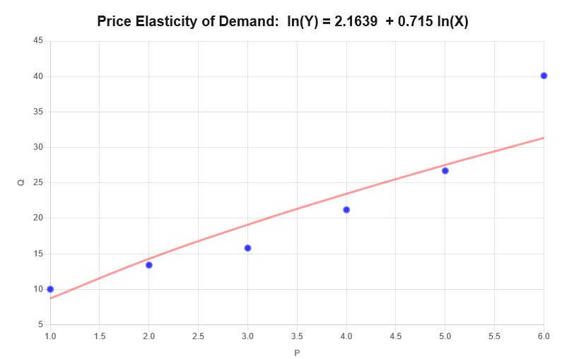
\[\ln(Q) = 2.1639 + 0.715 \ln(P)\]

Therefore, based on the information provided above, the following scatter plot and regression plot are obtained:

Interpretation

The elasticity in this case corresponds to the slope coefficient for the data provided, which means that \(\varepsilon = 0.715 \), which can be interpreted as follows:

• For an increase of 1% in price, there is an average increase of 0.715% in quantity demanded.

More Interesting Calculators

Estimating models from sample data is a crucial ability needed in both Statistics and Economics. Using sample data to compute a regression model is one of the most common applications of using sample data for model building.

But it is often the case that a regular linear model won't fit the data sufficiently well, for which we need to attempt different functional structures. For example, we could potentially estimate a log-log regression, a logarithmic regression or a polynomial regression, just to mention a few, which could be more successful at explaining the variation in the dependent variable than regular regression.

The option of computing the elasticity from sample data is mostly used in an exploratory setting. More often than not, the elasticity is directly computed from the demand function, when available. In other circumstances, the elasticity is estimated from a pair of price-demand points using the arc-elasticity formula.