Question 1: Linear Regression Formula The formulas for the least square line were found by solving the system of equations

\[nb+m\left( \sum{x} \right)=\sum{y}\]

\[b\left( \sum{x} \right)+m\left( \sum{x^2} \right)=\sum{xy}\]

How do you calculate linear regression by hand? Solve these equations for b and m to show that

\[\begin{align} & m=\frac{n\left( \sum{xy} \right)-\left( \sum{x} \right)\left( \sum{y} \right)}{n\left(\sum{{{x}^{2}}} \right)-{{\left( \sum{x} \right)}^{2}}} \\ & b=\frac{\sum{y-m\left( \sum{x}\right)}}{n} \\ \end{align}\]

Solution: From

\[ nb+m\left( \sum{x} \right)=\sum{y}\]

\[b\left( \sum{x} \right)+m\left( \sum{x^2} \right)=\sum{xy}\]

we have two equations and two unknowns (m and b)

We get that multiplying the first equation by \(\left( \sum{x} \right)\) and the second by -n we get

\[\begin{align} & nb\left( \sum{x} \right)+m{{\left( \sum{x} \right)}^{2}}=\left( \sum{y}\right)\left(\sum{x} \right) \\ & -nb\left( \sum{x} \right)-mn\left( {{\sum{x}}^{2}}\right)=n\sum{xy} \\ \end{align}\]

and now adding these:

\[m\left( {{\left( \sum{x} \right)}^{2}}-n\left( {{\sum{x}}^{2}} \right) \right)=\left( \sum{x} \right)\left(\sum{y} \right)-n\left( \sum{xy} \right)\]

\[\Rightarrow \,\,\,\,m=\frac{\left( \sum{x} \right)\left( \sum{y} \right)-n\left( \sum{xy} \right)}{{{\left( \sum{x} \right)}^{2}}-n\left( {{\sum{x}}^{2}} \right)}=\frac{n\left( \sum{xy} \right)-\left( \sum{x} \right)\left( \sum{y} \right)}{n\left( {{\sum{x}}^{2}} \right)-{{\left( \sum{x} \right)}^{2}}}\]

Now, from this equation:

\[nb+m\left( \sum{x} \right)=\left( \sum{y} \right)\]

we can solve for b :

\[nb+m\left( \sum{x} \right)=\left( \sum{y} \right)\,\,\Rightarrow \,\,\,nb=\left( \sum{y} \right)-m\left( \sum{x} \right)\,\Rightarrow \,\,\,b=\frac{\left( \sum{y} \right)-m\left( \sum{x} \right)}{n}\]

Question 2: Determine the correlation coefficient and do a graph of the regression line with the regression coefficient for the following set of data.

Forest fires and acres burned. The number of fires and the number of acres burned are as follows

Fires (x)	72	69	58	47	84	62	57	45
Acres(y)	62	41	19	26	51	15	30	15

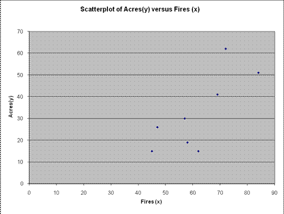
Solution: (a) The following scatterplot is obtained:

Based on the scatterplot above, we observe that there is a moderate to strong degree of positive linear association.

(b) On the other hand, we have the following table shows the calculations needed in order to compute Pearson correlation: We get

The Pearson correlation r is computed as

\[r = \frac{n\sum\limits_{i=1}^{n}{{{x}_{i}}{{y}_{i}}}-\left( \sum\limits_{i=1}^{n}{{{x}_{i}}} \right)\left( \sum\limits_{i=1}^{n}{{{y}_{i}}} \right)}{\sqrt{n\left( \sum\limits_{i=1}^{n}{x_{i}^{2}} \right)-{{\left( \sum\limits_{i=1}^{n}{{{x}_{i}}} \right)}^{2}}}\sqrt{n\left( \sum\limits_{i=1}^{n}{y_{i}^{2}} \right)-{{\left( \sum\limits_{i=1}^{n}{{{y}_{i}}} \right)}^{2}}}} = \frac{8 \times {17216}-{494}\times {259}}{\sqrt{8\times {31692}-{494}^{2}}\sqrt{8\times 10513-{259}^{2}}}\]

\[=0.7692\]

(c) The coefficient of determination is

\[{{r}^{2}}={0.7692}^{2}= {0.5917}\]

which means that 59.17% of the variation in Acres(y) is explained by Fires (x) .

(d) We need to calculate the regression equation. The regression coefficients are computed

\[b=\frac{n\left( \sum\limits_{i=1}^{n}{{{x}_{i}}{{y}_{i}}} \right)-\left( \sum\limits_{i=1}^{n}{{{x}_{i}}} \right)\left( \sum\limits_{i=1}^{n}{{{y}_{i}}} \right)}{n\left( \sum\limits_{i=1}^{n}{x_{i}^{2}} \right)-{{\left( \sum\limits_{i=1}^{n}{{{x}_{i}}} \right)}^{2}}}=\frac{8 \times {17216}-{494}\times {259}}{8 \times {31692}-{494}^{2}}= 1.0297\]

and

\[a=\bar{y}-b \bar{x}={32.375}{+} {1.0297}\,\cdot \, {61.75} = {-31.208}\]

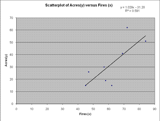
This means that the regression equation is

\[\hat{y}= {-31.208}{+}{1.0297}\,x\]

Graphically:

Question 3: You have conducted a study to determine if the average time spent in the computer lab each week and the course grade in a computer course were correlated. Using the data given below, what conclusion would you draw on this issue?

student	# hours in lab	Course Grade
1	20	96
2	11	51
3	16	62
4	13	58
5	89
6	15	81
7	10	46
8	10	51

Solution: The following table shows the calculations needed in order to compute Pearson correlation r : We get

The Pearson correlation r is computed as

\[r = \frac{n\sum\limits_{i=1}^{n}{{{x}_{i}}{{y}_{i}}}-\left( \sum\limits_{i=1}^{n}{{{x}_{i}}} \right)\left( \sum\limits_{i=1}^{n}{{{y}_{i}}} \right)}{\sqrt{n\left( \sum\limits_{i=1}^{n}{x_{i}^{2}} \right)-{{\left( \sum\limits_{i=1}^{n}{{{x}_{i}}} \right)}^{2}}}\sqrt{n\left( \sum\limits_{i=1}^{n}{y_{i}^{2}} \right)-{{\left( \sum\limits_{i=1}^{n}{{{y}_{i}}} \right)}^{2}}}} = \frac{8 \times {7925}-{112}\times {534}}{\sqrt{8\times {1660}-{112}^{2}}\sqrt{8\times 38224-{534}^{2}}}\]

\[=0.9217\]

We want to test for the significance of the correlation coefficient. More specifically, we want to test

\[\begin{align}{{H}_{0}}:\rho {=} 0 \\ {{H}_{A}}:\rho {\ne} 0 \\ \end{align}\]

In order to test the null hypothesis, we use a t-test. The t-statistics is computed as

\[t= r \sqrt{\frac{n-2}{1-{{r}^{2}}}}= {0.9217} \times \sqrt{\frac{6}{1-{0.9217}^2}}= {5.8198}\]

The two-tailed p-value for this test is computed as

\[p=\Pr \left( |{{t}_{6}}|>5.8198 \right)=0.0011\]

Since \(p = 0.0011 {<} 0.05\) , and this means that we reject the null hypothesis H ₀ .

Hence, we have enough evidence to support the claim that the correlation between Number of hours in lab and Course Grade is significantly different from zero.

Since there is sufficient evidence to assume that there is a meaningful linear association, you can now use this regression equation calculator to estimate its regression coefficients, or you can calculate the regression coefficients by hand using the formula presented above.