The Mean, the Median and the Mode are the most common measures of central tendency, used to describe the center of a distribution. Out of the three, the mean is the most commonly used one, but the median and mode are also widely used.
![]() We need to distinguish between the
sample
mean, median and mode, and their
population
counterparts.
We need to distinguish between the
sample
mean, median and mode, and their
population
counterparts.
![]() Typically, we are
provided with a sample
and we need to compute the sample mean, the sample median and the sample mode. These statistics are
estimators
of the corresponding population parameters.
Typically, we are
provided with a sample
and we need to compute the sample mean, the sample median and the sample mode. These statistics are
estimators
of the corresponding population parameters.
In the graph above you have an example of a how the median, mode and mean would look in a distribution.
![]() The mode corresponds to the most repeated value in a sample. In a distribution, it corresponds to the highest point in the density function, as shown in the graph above.
The mode corresponds to the most repeated value in a sample. In a distribution, it corresponds to the highest point in the density function, as shown in the graph above.
![]() The median, roughly, defines the point where 50% of the distribution lies to left of it, and to the right of it.
The median, roughly, defines the point where 50% of the distribution lies to left of it, and to the right of it.
![]() The mean corresponds to the weighted average of the values that the variable takes and their associated probabilities (\(\sum x \cdot p(x)\)). For a distribution, such weighted sum is either a summation or an integral. For a sample, we just compute simply the average of values in the sample.
The mean corresponds to the weighted average of the values that the variable takes and their associated probabilities (\(\sum x \cdot p(x)\)). For a distribution, such weighted sum is either a summation or an integral. For a sample, we just compute simply the average of values in the sample.
How to Compute the Mean, Median and Mode for a Given Sample
Now, assume that we are given a sample \(X_1, X_2, ..., X_n\), and we want to compute the mode, median and mean. How do we go about it?
• For the Mode: Simple. We just find the number that is the most repeated. Ex: If we have a sample 1, 2, 2, 2, 3, 1, 4, the mode is 2, because 2 is the most repeated value (it is repeated 3 times)
• For the Median: This calculation is slightly more involved. Take your sample \(X_1, X_2, ..., X_n\) and the first step is to reorganize it in ascending order. So, assume that \(\hat X_1, \hat X_2, ..., \hat X_n\) is the sample after reordering it from lowest to highest values.
Now, we are going to compute the position of the median in the sample in ascending order. For the sample size \(n\), we compute \(P = 0.5 (n+1)\).
![]() If this value is an integer, then we find that the median is the value in the P
th
position in the sample in ascending order.
If this value is an integer, then we find that the median is the value in the P
th
position in the sample in ascending order.
![]() If this value is NOT integer, then we find \(P_L\) and \(P_U\) which are the closest integers to the left and right of \(P\). (Ex: If \(P = 10.2\), then \(P_L = 10\) and \(P_U = 11\)).
If this value is NOT integer, then we find \(P_L\) and \(P_U\) which are the closest integers to the left and right of \(P\). (Ex: If \(P = 10.2\), then \(P_L = 10\) and \(P_U = 11\)).
Then, the median is the average of values that are in positions \(P_L\) th and \(P_U\) th in the sample in ascending order. Don't worry, we will practice this with an example.
• For the Mean: Simple as well. The sample mean is calculated by using the formula
\[\displaystyle \frac{1}{n}\sum_{i=1}^n X_i\]EXAMPLE 1
Find the mean, median and mode for the following sample:
28, 36, 43, 30, 15, 19, 46, 36, 34, 38, 42, 29, 37, 35, 39, 39, 30, 39, 36, 38, 30, 41, 42, 46, 40, 33, 30, 40, 43, 12 42, 39, 30, 35, 38, 41, 30, 37, 40, 30, 30, 35, 39, 37, 42, 42, 37, 38, 32, 51
ANSWER:
The following table shows the required calculations needed to compute the mean
|
Data |
|
|
28 |
|
|
36 |
|
|
43 |
|
|
30 |
|
|
15 |
|
|
19 |
|
|
46 |
|
|
36 |
|
|
34 |
|
|
38 |
|
|
42 |
|
|
29 |
|
|
37 |
|
|
35 |
|
|
39 |
|
|
39 |
|
|
30 |
|
|
39 |
|
|
36 |
|
|
38 |
|
|
30 |
|
|
41 |
|
|
42 |
|
|
46 |
|
|
40 |
|
|
33 |
|
|
30 |
|
|
40 |
|
|
43 |
|
|
12 |
|
|
42 |
|
|
39 |
|
|
30 |
|
|
35 |
|
|
38 |
|
|
41 |
|
|
30 |
|
|
37 |
|
|
40 |
|
|
30 |
|
|
30 |
|
|
35 |
|
|
39 |
|
|
37 |
|
|
42 |
|
|
42 |
|
|
37 |
|
|
38 |
|
|
32 |
|
|
51 |
|
|
Sum = |
1791 |
|
Mean = |
35.82 |
The sample mean is therefore
\[\bar{X}=\frac{1}{n}\sum{{{X}_{i}}}=\frac{1791}{50}=35.82\]Now for the median following table shows the data in ascending order:
|
Data (In ascending order) |
|
12 |
|
15 |
|
19 |
|
28 |
|
29 |
|
30 |
|
30 |
|
30 |
|
30 |
|
30 |
|
30 |
|
30 |
|
30 |
|
32 |
|
33 |
|
34 |
|
35 |
|
35 |
|
35 |
|
36 |
|
36 |
|
36 |
|
37 |
|
37 |
|
37 |
|
37 |
|
38 |
|
38 |
|
38 |
|
38 |
|
39 |
|
39 |
|
39 |
|
39 |
|
39 |
|
40 |
|
40 |
|
40 |
|
41 |
|
41 |
|
42 |
|
42 |
|
42 |
|
42 |
|
42 |
|
43 |
|
43 |
|
46 |
|
46 |
|
51 |
In this case, the position of the median is P = 0.5*(50+1) = 25.5, so then \({{P}_{L}}=25\) and \({{P}_{U}}=26\). The value in position 25 th in the data in ascending order is 37, and the value in position 26th is 37 as well. The median is then
\[Median=\frac{{37}+{37}}{2}=37\]The mode, which is the most repeated value, is 30.
What is larger, the mean, median or mode?
That is a question that pops up frequently. In general terms, there is not one answer for all distributions. This is, the answer depends on the distribution.
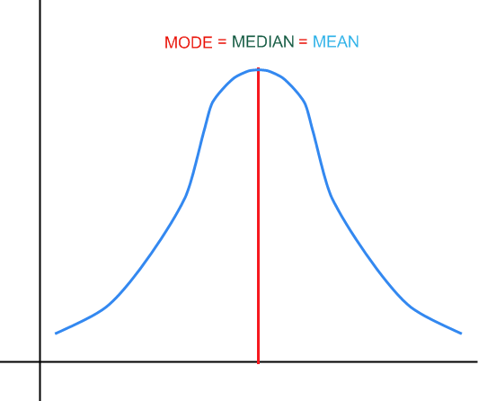
![]() For a symmetric distribution we have
:
For a symmetric distribution we have
:
Graphically:
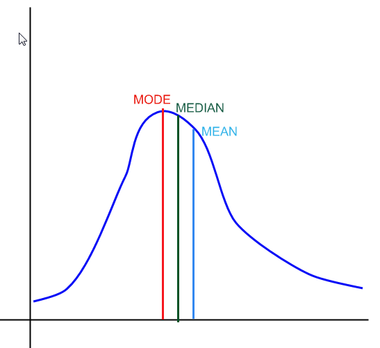
![]() For a right-skewed distribution we have
:
For a right-skewed distribution we have
:
Graphically:
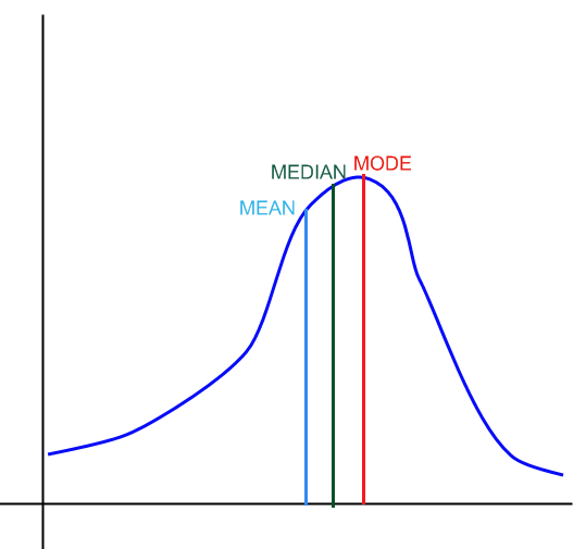
![]() For a left-skewed distribution we have
:
For a left-skewed distribution we have
:
Graphically:
More About the Mean, Median and Mode
The median, mean and mode are broadly popular concepts that are used everywhere in Statistics. They represent measures of center, which attempt to give a value that is representative of the sample.
Depending on the level of measurement, we would use a different measure of center.
• For nominal data, we use the mode.
• For ordinal, non-quantitative data we use the mode as well as the measure of center.
• For ordinal, quantitative data we use the median or the mean as the measure of center.
• For interval and ratio data, we use the mean (or the median if the distribution is too skewed) as the measure of center.
Applications
The mean, median and mode are the most typically used measures of center. The mean and median are used for quantitative data, and the mode is used for categorical data.
For quantitative data, one would typically use the mean. With one caveat: the mean is very sensitive to outliers. This means that one outlier (either legitimate value or a typing error) could make a drastic difference on the value of the mean.
In such cases, when there are outliers or the distribution is fairly skewed, it is preferable to use the median as the most accurate measure of center, because the mean gets distorted by skewness or outliers.
One example of this is when samples are collected to assess income of the respondents. If we take a sample of 100 people, and we find that 99 of them make $10,000 per year, and 1 person makes $100 million per year, the average income of that sample would be (10,000*99 + 1*100,000,000)/100 = $1,009,900.00. So, on average, everyone makes $1,009,900.00, so you would get the idea that this sample must come from a very affluent area, but that is not the case: it is just one outlier highly distorting the mean. Indeed, in this case, the median is $10,000, which is a much more representative value of center for this sample.
Related Calculators
If you need to see step-by-step solutions for the calculation of the mean and other measures of central tendency, check out descriptive statistics calculator . You can also find useful our 5-number summary calculator .
Related Posts:
-
 Free Math Help Resources
-
Partial Fraction Decomposition
-
Substitution Method of Integration
-
Gaussian Elimination
-
Box and Whisker Plot
-
Exponential Decay Formula
-
Absolute Value Inequalities
-
Functions: What They Are and How to Deal with Them


In case you have any suggestion, or if you would like to report a broken solver/calculator, please do not hesitate to contact us .