Gaussian Elimination is a process conducted on matrices aimed to put a matrix into echelon form . Having a matrix in such form helps enormously to solving matrix equations very easily.

Technically, the process of conducting Gaussian elimination consists in finding a column with a pivot (which is the fancy slang for a non-zero element) that allows us to eliminate all the elements below the pivot.

This process of finding pivots and eliminating allows us to put a matrix into echelon form, and the way the process goes is such that by pivoting you add a new column to the echelon form, and you don't 'ruin' the echelon form you have made up to the previous step. Beautiful if you ask me.

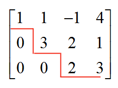
The term "echelon form" that is obtained by using Gaussian elimination becomes clear by looking at the matrix above, where the non-zero elements of the matrix have this echelon-like structure, as shown by the red line.

The Math Behind Pivoting and Gaussian Elimination

We are not going to get too technical into this, we only are going to try that you understand the motivation and the mechanics of this kind of elimination.

The idea is to get a matrix \(A\), of dimension \(m \times n\) (this is, it has \(m\) rows and \(n\) columns) into a different form that is more amenable for solving equations.

More specifically, for a \(m\times n\) matrix \(A\), and a \(m\times 1\) vector \(b\), we need to find a \(n\times 1\) vector \(x\) such that

You may think, "that is so easy, we just multiply each side by \(A^{-1}\) from the left" so we get:

....Not so fast! That only works when the matrix \(A\) is invertible. To start, the matrix \(A\) has to be a square matrix, and then, its determinant needs to be different from zero. But you cannot multiply by the inverse for non-square matrices. So, how do you do it then?

You need to TRANSFORM the equation into one that is easier to solve.

Specifically, matrices in echelon form are matrices that lead to equations that are easy to solve (more about that later).

Using Elementary Matrices

First of all, we will make a crucial note. If we have a solution of the matrix equation \(Ax = b\), and \(E\) is an invertible matrix, then \(x\) is also a solution of \((EA)x = Eb\), and vice versa.

In other words, the matrix equations

and

are equivalent, for an invertible matrix \(E\). What do we mean by that the equations are equivalent? We mean that the equations have the same solutions.

So what we are going to do is to start with \(Ax = b\), and via multiplying by invertible matrices \(E\), we are going to arrive to an equivalent matrix equation that is much easier to solve .

Say that we are able to find a list of invertible matrices \(E_1, E_2, ..., E_n\) and we multiply (from the left) the original matrix equation to transform it into an equivalent equation, like:

where \(E_n \cdots E_2 \cdot E_1 \cdot A = \tilde A\) and \(E_n \cdots E_2 \cdot E_1 \cdot A = \tilde b\).

Our aim is to carefully choose the invertible matrices \(E_1, E_2, ..., E_n\) so that \(\tilde A\) is in echelon form.

Why is that? Because if \(\tilde A\) is in echelon form, solving the matrix equation \(\tilde A x = \tilde b\) is much easier, and we already know that \(\tilde A x = \tilde b\) has the same solutions as \(A x = b\)

EXAMPLE 1

Let us see why solving a matrix equation is much easier when you have it in echelon form. First imagine that you have the following matrix and vector:

and you want to solve \(Ax = b\). How would the system of equations look? The system \(Ax = b\) would look like

How does it look? Well, not that neat. You would need to start juggling equations. There are more or less systematic approaches to solve this using things like elimination and such, but it is at least cumbersome.

Now, on the other hand, imagine that you have the following matrix and vector:

and you want to solve \(\tilde A x = \tilde b\). In this case, the matrix \(\tilde A\) is in echelon form. How would the system of equations look? The system \(\tilde A x = \tilde b\) would look like

How does this one look? Well, not too shabby.

Indeed, if we start directly from the third equation, we have that \(x_3 = -1\) directly. Then from the second equation, \(x_2 = -1 + x_3 = -1 + (-1) = -2\). And from the first equation, \(x_1 = x_2 + x_3 -1 = -2 + (-1) - 1 = -4\). So without any fuzz, we have found that:

Therefore, in this case the system is solved trivially.

For systems associated to matrices in echelon form, it is straightforward to backtrack from the last equation to the first equation, to get the solutions.

How to Choose the Right Invertible Matrices

Now that we know that working with matrices in echelon form makes it really much easier to solve matrix equations, we should be wondering, what are the invertible matrices \(E_1, E_2, ..., E_n\) that will make \(\tilde A\) in echelon form.

How does Gaussian elimination work?

Interestingly enough, it is not hard to find these matrices \(E_1, E_2, ..., E_n\), which will be called elementary matrices.

Step 1 : Look at the first column, if it has a non-zero value, that will be your pivot. If the first row of the first column is non-zero, use it as pivot. If not, find a row that has a non-zero value and permute that row and the first row.

So, you find a pivot, and potentially you need to make a row permutation (which is actually represented by multiplying by a certain an invertible matrix)

Step 2 : Once you have a pivot, eliminate all the elements in the current column, below the pivot.

This is done by multiplying the pivot row by a certain constant, and adding that to a row below the pivot, so that the element in the same column as the pivot is made zero.

Step 3 : Once all the elements below the pivot have been made zero by making appropriate row operations (which happen to be represented by the operation of an invertible matrix), move to the next column, next row, and look for a pivot from the row below of the row of the previous pivot and make the same procedure.

Step 4 : Repeat until you run out of columns or the matrix is in echelon form.

EXAMPLE 2

Using pivoting and Gaussian elimination, solve the following system:

ANSWER:

First of all, the associated matrix \(A\) and vector \(b\) are:

The augmented matrix \([A|b]\) is

In order to solve the system, we need to go gaussian elimination. We choose the first pivot, starting with the first column. The element in the first row of the first column is 1, which is different from zero and then, it is used as a pivot. We use that pivot (1) to eliminate all the elements below it:

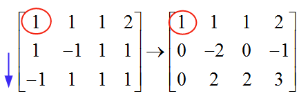
The mechanic of eliminating the elements below the pivot is simple. In this case, to eliminate the "1" that is below the pivot, I subtract the elements in row 1 to the elements in row 2. That way I form a zero under the pivot.

Similarly, to eliminate the "-1" that is in row 3, I add the elements in row 1 to the elements in row 3. That way I form a zero under the pivot in row 3.

We will see that this row operations are achieved by multiplying by invertible matrix, so we have equivalent systems by doing so.

Now, moving to the next row, next column, we find a "-2", which is different from zero, and hence, it is used as our pivot. To eliminate the value below this pivot, we add to row 3 the values of row 2:

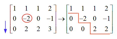
and now we stop, because the resulting matrix is already in echelon form. Now we back-track to solve the system: