Synthetic Division of Polynomials

This calculator will allow you to do a synthetic division of two polynomials. These polynomials can be anything, but with one restriction: the divisor needs to have degree 1 in order to use this method.

So for example, you can type the first polynomial (the dividend) as '3x^3 + 2x^2 + 1', and the divisor could be for example 'x+1'.

The divisor needs to have degree 1. For example, valid divisors would be x+1 , 2x-1, etc, but x^2 + 1 would not be a valid divisor for synthetic division because it has degree 2.

The polynomials you provide do not need to be simplified necessarily, and if they are not, the calculator will do it before doing the division of the polynomials. Then, once you have provided two valid polynomials, you need to click on the "Calculate" button, in order to get all the steps of the calculation.

What is Synthetic Division

Synthetic division is a simplified procedure to divide polynomials. It applies to the specific case when the polynomial you are dividing by (the divisor) has degree equal to 1.

For example, the following polynomial division can be calculated using synthetic division:

\[\displaystyle \frac{2x^3+3x+1}{x+1} \]

because the divisor \(x+1\) has degree 1. Now the following division could not be computed using synthetic division:

\[\displaystyle \frac{x^4+ + 2x^2 + 2x+1}{x^2+1} \]

because the divisor \(x^2+1\) has degree 2. Technically, you could extend synthetic division for higher degrees, but its main goal is to be a quick division method for a linear divisor (a divisor with degree 1).

Synthetic Division versus Long Division

What is the difference between long and synthetic division? First of all, long division of polynomials can be applied to all polynomials, not only when the divisor has degree 1, but for all possible divisors, as long as they are valid polynomials.

So then, the advantage of polynomial long division is that it is a general method that applies to all possible polynomials, but then its disadvantage is that it tends to be more algebraically intensive.

The advantage of synthetic division is that it gives a quick division method (much simpler than long division), but its disadvantage is that it only applies to divisors of degree 1.

What are the steps for doing synthetic division of polynomials?

• Step 1: Name the polynomials you wish to divide as p(x) and s(x), with p(x) being the dividend and s(x) being the divisor. Ensure that both are polynomials before proceeding
• Step 2: Make sure that the degree of the divisor s(x) is 1. If not, stop, you cannot do synthetic division
• Step 3: Now, find the value of x for which s(x) = 0. This value will be placed in the 'division box'
• Step 4: Create a row with the coefficients of the dividend in it (higher powers first), and create two other empty rows: One will store the final results and one will store intermediate results
• Step 5: For the first column, you pass the dividend coefficient down to the results row, and the intermediate result is 0
• Step 6: For the following columns, you multiply the previous value in the results row by the value in the division box and store this value in the correspondent intermediate row. Then, add the dividend coefficient and this intermediate value to get the final value for the colum
• Step 7: Repeat the previous steps for the following columns

That is how you divide using synthetic division. It is an iteration of steps in which you go updating the rows until you get the coefficients of the quotient polynomial and the remainder, which in this case must be a number. For long division, the remainder can be a polynomial, but it will have lower degree than the divisor.

The synthetic division procedure as described above could be confusing, so the best way to go about is to see some examples.

Synthetic substitution calculator

It is important to mention that synthetic division is often times used for synthetic substitution, which is the technique that consists of evaluating a given value x = a on a polynomial p(x), without actually doing a traditional evaluation in the function, but by applying synthetic division, by virtue of the Remainder Theorem.

So, even though often times, running the steps of an iterative process can be confusing, this polynomial division calculator will be very helpful at showing you all the steps of the process described above, and can be used in multiple applications.

Now, if you want to divide using synthetic division manually, it is still possible and not too cumbersome, as opposed to what would be the case with division of polynomials using long division, which tends to involve a much more lengthy calculation.

Should I use synthetic or long division?

• Step 1: Clearly identify two polynomials you want to divide. Call p(x) to the dividend and s(x) to the divisor. Make sure they are polynomials, otherwise, you stop
• Step 2: Look at the divisor and find its degree
• Step 3: If the degree of the divisor is 1, use synthetic division, otherwise, use long division

One interesting feature of both synthetic and long division is that they achieve a division of polynomials by using sums and multiplications, which is pretty useful, because those are polynomial operations that are simple and straightforward to use.

Is there a synthetic division formula?

Not quite. The process of calculating synthetic divisions is based on an algorithm rather than a formula. An algorithm is a well defined process where different steps are being conducted, until the process is completed.

So, you won't have a synthetic division formula (although theoretically you put it an abstract way), but instead, you have a 'recipe' on how to do the steps.

Synthetic Division and root of polynomials

One of the most typical applications of synthetic division is for testing whether a number \(x = a\) is a root of a given polynomial \(p(x)\) or not. The way you do it is simple: You just apply synthetic division for the dividend \(p(x)\) and the divisor \(s(x) = x - a\). Then, if the remainder is 0, then number \(x = a\) is a root of the polynomial.

Also, if it is indeed a root, you get the quotient \(q(x)\) and then you have concluded that \(p(x) = q(x)(x-a)\), so then, in order to find the roots of \(p(x)\), you just need to find the roots of \(q(x)\), which has one degree less, so it should be easier.

Example: Synthetic division examples

Calculate the division : \(\displaystyle \frac{x^4+x^3+x^2+2}{x-1}\)

Solution:

The following polynomial has been provided: \(\displaystyle p(x) = x^4+x^3+x^2+2\), which needs to be divided by the polynomial \(\displaystyle s(x) = x-1\).

Observe that the degree of the dividend is \(\displaystyle deg(p) = 4\), whereas the degree of the divisor is \(\displaystyle deg(s)) = 1\).

Step 1: Since the divisor has a degree 1, we can use the Synthetic Division method. By solving \(\displaystyle s(x) = x-1 = 0\) we find directly that the number to put in the division box is: \(\displaystyle 1\).

\[\begin{array}{c|cccc} 1 & \displaystyle 1 & \displaystyle 1 & \displaystyle 1 & \displaystyle 0 & \displaystyle 2 \\[0.6em] & & & & & & \\[0.6em] \hline & & & & & & \end{array}\]

Step 2: Now we pass directly the leading term \(\displaystyle 1\) to the result row:

\[\begin{array}{c|cccc} 1 & \displaystyle 1 & \displaystyle 1 & \displaystyle 1 & \displaystyle 0 & \displaystyle 2 \\[0.6em] & & & & & & \\[0.6em] \hline &\displaystyle 1&&&& \end{array}\]

Step 3: Multiplying the term in the division box by the result in column 1: \(1 \cdot \left(1\right) = 1\) and this result is inserted in the result row, column1.

\[\begin{array}{c|cccc}1 & \displaystyle 1 & \displaystyle 1 & \displaystyle 1 & \displaystyle 0 & \displaystyle 2\\[0.6em]& 0 & 1 & & \\[0.6em]\hline&\displaystyle 1&&&&\end{array}\]

Step 4: Now adding the values in column 2: \( \displaystyle 1+1 = 2\) and this result is inserted in the result row, column2.

\[\begin{array}{c|cccc}1 & \displaystyle 1 & \displaystyle 1 & \displaystyle 1 & \displaystyle 0 & \displaystyle 2\\[0.6em]& 0 & 1 & & \\[0.6em]\hline& 1 & 2 & & \end{array}\]

Step 5: Multiplying the term in the division box by the result in column 2: \(1 \cdot \left(2\right) = 2\) and this result is inserted in the result row, column2.

\[\begin{array}{c|cccc}1 & \displaystyle 1 & \displaystyle 1 & \displaystyle 1 & \displaystyle 0 & \displaystyle 2\\[0.6em]& 0 & 1 & 2 & \\[0.6em]\hline& 1 & 2 & & \end{array}\]

Step 6: Now adding the values in column 3: \( \displaystyle 1+2 = 3\) and this result is inserted in the result row, column3.

\[\begin{array}{c|cccc}1 & \displaystyle 1 & \displaystyle 1 & \displaystyle 1 & \displaystyle 0 & \displaystyle 2\\[0.6em]& 0 & 1 & 2 & \\[0.6em]\hline& 1 & 2 & 3 & \end{array}\]

Step 7: Multiplying the term in the division box by the result in column 3: \(1 \cdot \left(3\right) = 3\) and this result is inserted in the result row, column3.

\[\begin{array}{c|cccc}1 & \displaystyle 1 & \displaystyle 1 & \displaystyle 1 & \displaystyle 0 & \displaystyle 2\\[0.6em]& 0 & 1 & 2 & 3\\[0.6em]\hline& 1 & 2 & 3 & \end{array}\]

Step 8: Now adding the values in column 4: \( \displaystyle 0+3 = 3\) and this result is inserted in the result row, column4.

\[\begin{array}{c|cccc}1 & \displaystyle 1 & \displaystyle 1 & \displaystyle 1 & \displaystyle 0 & \displaystyle 2\\[0.6em]& 0 & 1 & 2 & 3\\[0.6em]\hline& 1 & 2 & 3 & 3\end{array}\]

Step 9: Multiplying the term in the division box by the result in column 4: \(1 \cdot \left(3\right) = 3\) and this result is inserted in the result row, column4.

\[\begin{array}{c|cccc}1 & \displaystyle 1 & \displaystyle 1 & \displaystyle 1 & \displaystyle 0 & \displaystyle 2\\[0.6em]& 0 & 1 & 2 & 3 & 3\\[0.6em]\hline& 1 & 2 & 3 & 3\end{array}\]

Step 10: Now adding the values in column 5: \( \displaystyle 2+3 = 5\) and this result is inserted in the result row, column5.

\[\begin{array}{c|cccc}1 & \displaystyle 1 & \displaystyle 1 & \displaystyle 1 & \displaystyle 0 & \displaystyle 2\\[0.6em]& 0 & 1 & 2 & 3 & 3\\[0.6em]\hline& 1 & 2 & 3 & 3 & 5\end{array}\]

which concludes this calculation, since we have arrived to the result in the final column, which contains the remainder.

Conclusion: Therefore, we conclude that for the given dividend \(\displaystyle p(x) = x^4+x^3+x^2+2\) and divisor \(\displaystyle s(x) = x-1\), we get that the quotient is \(\displaystyle q(x) = x^{ 3}+2 x^{ 2}+3 x+3\) and the remainder is \(\displaystyle r(x) = 5\), and that

\[\displaystyle \frac{p(x)}{s(x)} = \frac{x^4+x^3+x^2+2}{x-1} = x^{ 3}+2 x^{ 2}+3 x+3 + \frac{5}{x-1}\]

Example: Example of synthetic division

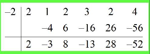
Do the following division of polynomials : \(\displaystyle \frac{x^5+x^3+x^2+2}{x-2}\)

Is \(x = 2\) a root of the polynomial \(x^5+x^3+x^2+2\)?

Solution:So in this case, we take the polynomial \(\displaystyle p(x) = x^5+x^3+x^2+2\) and we divide it by \(\displaystyle s(x) = x-2\).

The objective is to see whether or not the remainder is zero.

Step 1: Since the divisor has a degree 1, we can use the Synthetic Division method. By solving \(\displaystyle s(x) = x-2 = 0\) we find directly that the number to put in the division box is: \(\displaystyle 2\).

\[\begin{array}{c|ccccc} 2 & \displaystyle 1 & \displaystyle 0 & \displaystyle 1 & \displaystyle 1 & \displaystyle 0 & \displaystyle 2 \\[0.6em] & & & & & & & \\[0.6em] \hline & & & & & & & \end{array}\]

Step 2: Now we pass directly the leading term \(\displaystyle 1\) to the result row:

\[\begin{array}{c|ccccc} 2 & \displaystyle 1 & \displaystyle 0 & \displaystyle 1 & \displaystyle 1 & \displaystyle 0 & \displaystyle 2 \\[0.6em] & & & & & & & \\[0.6em] \hline &\displaystyle 1&&&&& \end{array}\]

Step 3: Multiplying the term in the division box by the result in column 1: \(2 \cdot \left(1\right) = 2\) and this result is inserted in the result row, column1.

\[\begin{array}{c|ccccc}2 & \displaystyle 1 & \displaystyle 0 & \displaystyle 1 & \displaystyle 1 & \displaystyle 0 & \displaystyle 2\\[0.6em]& 0 & 2 & & & \\[0.6em]\hline&\displaystyle 1&&&&&\end{array}\]

Step 4: Now adding the values in column 2: \( \displaystyle 0+2 = 2\) and this result is inserted in the result row, column2.

\[\begin{array}{c|ccccc}2 & \displaystyle 1 & \displaystyle 0 & \displaystyle 1 & \displaystyle 1 & \displaystyle 0 & \displaystyle 2\\[0.6em]& 0 & 2 & & & \\[0.6em]\hline& 1 & 2 & & & \end{array}\]

Step 5: Multiplying the term in the division box by the result in column 2: \(2 \cdot \left(2\right) = 4\) and this result is inserted in the result row, column2.

\[\begin{array}{c|ccccc}2 & \displaystyle 1 & \displaystyle 0 & \displaystyle 1 & \displaystyle 1 & \displaystyle 0 & \displaystyle 2\\[0.6em]& 0 & 2 & 4 & & \\[0.6em]\hline& 1 & 2 & & & \end{array}\]

Step 6: Now adding the values in column 3: \( \displaystyle 1+4 = 5\) and this result is inserted in the result row, column3.

\[\begin{array}{c|ccccc}2 & \displaystyle 1 & \displaystyle 0 & \displaystyle 1 & \displaystyle 1 & \displaystyle 0 & \displaystyle 2\\[0.6em]& 0 & 2 & 4 & & \\[0.6em]\hline& 1 & 2 & 5 & & \end{array}\]

Step 7: Multiplying the term in the division box by the result in column 3: \(2 \cdot \left(5\right) = 10\) and this result is inserted in the result row, column3.

\[\begin{array}{c|ccccc}2 & \displaystyle 1 & \displaystyle 0 & \displaystyle 1 & \displaystyle 1 & \displaystyle 0 & \displaystyle 2\\[0.6em]& 0 & 2 & 4 & 10 & \\[0.6em]\hline& 1 & 2 & 5 & & \end{array}\]

Step 8: Now adding the values in column 4: \( \displaystyle 1+10 = 11\) and this result is inserted in the result row, column4.

\[\begin{array}{c|ccccc}2 & \displaystyle 1 & \displaystyle 0 & \displaystyle 1 & \displaystyle 1 & \displaystyle 0 & \displaystyle 2\\[0.6em]& 0 & 2 & 4 & 10 & \\[0.6em]\hline& 1 & 2 & 5 & 11 & \end{array}\]

Step 9: Multiplying the term in the division box by the result in column 4: \(2 \cdot \left(11\right) = 22\) and this result is inserted in the result row, column4.

\[\begin{array}{c|ccccc}2 & \displaystyle 1 & \displaystyle 0 & \displaystyle 1 & \displaystyle 1 & \displaystyle 0 & \displaystyle 2\\[0.6em]& 0 & 2 & 4 & 10 & 22\\[0.6em]\hline& 1 & 2 & 5 & 11 & \end{array}\]

Step 10: Now adding the values in column 5: \( \displaystyle 0+22 = 22\) and this result is inserted in the result row, column5.

\[\begin{array}{c|ccccc}2 & \displaystyle 1 & \displaystyle 0 & \displaystyle 1 & \displaystyle 1 & \displaystyle 0 & \displaystyle 2\\[0.6em]& 0 & 2 & 4 & 10 & 22\\[0.6em]\hline& 1 & 2 & 5 & 11 & 22\end{array}\]

Step 11: Multiplying the term in the division box by the result in column 5: \(2 \cdot \left(22\right) = 44\) and this result is inserted in the result row, column5.

\[\begin{array}{c|ccccc}2 & \displaystyle 1 & \displaystyle 0 & \displaystyle 1 & \displaystyle 1 & \displaystyle 0 & \displaystyle 2\\[0.6em]& 0 & 2 & 4 & 10 & 22 & 44\\[0.6em]\hline& 1 & 2 & 5 & 11 & 22\end{array}\]

Step 12: Now adding the values in column 6: \( \displaystyle 2+44 = 46\) and this result is inserted in the result row, column6.

\[\begin{array}{c|ccccc}2 & \displaystyle 1 & \displaystyle 0 & \displaystyle 1 & \displaystyle 1 & \displaystyle 0 & \displaystyle 2\\[0.6em]& 0 & 2 & 4 & 10 & 22 & 44\\[0.6em]\hline& 1 & 2 & 5 & 11 & 22 & 46\end{array}\]

Conclusion: Therefore, we conclude that for the given dividend \(\displaystyle p(x) = x^5+x^3+x^2+2\) and divisor \(\displaystyle s(x) = x-2\), we get that the quotient is \(\displaystyle q(x) = x^{ 4}+2 x^{ 3}+5 x^{ 2}+11 x+22\) and the remainder is \(\displaystyle r(x) = 46\), and that since the remainder is not zero, we conclude that \(x = 2\) is NOT a root of the polynomial \(x^5+x^3+x^2+2\).

Example: Does it divide it?

Indicate whether or not the polynomial \(x^5 - 19x^4 + 137x^3 - 461x^2 + 702x - 360\) is divided exactly by \(x-1\).

Solution:We are given the dividend \(\displaystyle p(x) = x^5-19x^4+137x^3-461x^2+702x-360\), and the division \(\displaystyle s(x) = x-1\).

Step 1: Since the divisor has a degree 1, we can use the Synthetic Division method. By solving \(\displaystyle s(x) = x-1 = 0\) we find directly that the number to put in the division box is: \(\displaystyle 1\).

\[\begin{array}{c|ccccc} 1 & \displaystyle 1 & \displaystyle -19 & \displaystyle 137 & \displaystyle -461 & \displaystyle 702 & \displaystyle -360 \\[0.6em] & & & & & & & \\[0.6em] \hline & & & & & & & \end{array}\]

Step 2: Now we pass directly the leading term \(\displaystyle 1\) to the result row:

\[\begin{array}{c|ccccc} 1 & \displaystyle 1 & \displaystyle -19 & \displaystyle 137 & \displaystyle -461 & \displaystyle 702 & \displaystyle -360 \\[0.6em] & & & & & & & \\[0.6em] \hline &\displaystyle 1&&&&& \end{array}\]

Step 3: Multiplying the term in the division box by the result in column 1: \(1 \cdot \left(1\right) = 1\) and this result is inserted in the result row, column1.

\[\begin{array}{c|ccccc}1 & \displaystyle 1 & \displaystyle -19 & \displaystyle 137 & \displaystyle -461 & \displaystyle 702 & \displaystyle -360\\[0.6em]& 0 & 1 & & & \\[0.6em]\hline&\displaystyle 1&&&&&\end{array}\]

Step 4: Now adding the values in column 2: \( \displaystyle -19+1 = -18\) and this result is inserted in the result row, column2.

\[\begin{array}{c|ccccc}1 & \displaystyle 1 & \displaystyle -19 & \displaystyle 137 & \displaystyle -461 & \displaystyle 702 & \displaystyle -360\\[0.6em]& 0 & 1 & & & \\[0.6em]\hline& 1 & -18 & & & \end{array}\]

Step 5: Multiplying the term in the division box by the result in column 2: \(1 \cdot \left(-18\right) = -18\) and this result is inserted in the result row, column2.

\[\begin{array}{c|ccccc}1 & \displaystyle 1 & \displaystyle -19 & \displaystyle 137 & \displaystyle -461 & \displaystyle 702 & \displaystyle -360\\[0.6em]& 0 & 1 & -18 & & \\[0.6em]\hline& 1 & -18 & & & \end{array}\]

Step 6: Now adding the values in column 3: \( \displaystyle 137-18 = 119\) and this result is inserted in the result row, column3.

\[\begin{array}{c|ccccc}1 & \displaystyle 1 & \displaystyle -19 & \displaystyle 137 & \displaystyle -461 & \displaystyle 702 & \displaystyle -360\\[0.6em]& 0 & 1 & -18 & & \\[0.6em]\hline& 1 & -18 & 119 & & \end{array}\]

Step 7: Multiplying the term in the division box by the result in column 3: \(1 \cdot \left(119\right) = 119\) and this result is inserted in the result row, column3.

\[\begin{array}{c|ccccc}1 & \displaystyle 1 & \displaystyle -19 & \displaystyle 137 & \displaystyle -461 & \displaystyle 702 & \displaystyle -360\\[0.6em]& 0 & 1 & -18 & 119 & \\[0.6em]\hline& 1 & -18 & 119 & & \end{array}\]

Step 8: Now adding the values in column 4: \( \displaystyle -461+119 = -342\) and this result is inserted in the result row, column4.

\[\begin{array}{c|ccccc}1 & \displaystyle 1 & \displaystyle -19 & \displaystyle 137 & \displaystyle -461 & \displaystyle 702 & \displaystyle -360\\[0.6em]& 0 & 1 & -18 & 119 & \\[0.6em]\hline& 1 & -18 & 119 & -342 & \end{array}\]

Step 9: Multiplying the term in the division box by the result in column 4: \(1 \cdot \left(-342\right) = -342\) and this result is inserted in the result row, column4.

\[\begin{array}{c|ccccc}1 & \displaystyle 1 & \displaystyle -19 & \displaystyle 137 & \displaystyle -461 & \displaystyle 702 & \displaystyle -360\\[0.6em]& 0 & 1 & -18 & 119 & -342\\[0.6em]\hline& 1 & -18 & 119 & -342 & \end{array}\]

Step 10: Now adding the values in column 5: \( \displaystyle 702-342 = 360\) and this result is inserted in the result row, column5.

\[\begin{array}{c|ccccc}1 & \displaystyle 1 & \displaystyle -19 & \displaystyle 137 & \displaystyle -461 & \displaystyle 702 & \displaystyle -360\\[0.6em]& 0 & 1 & -18 & 119 & -342\\[0.6em]\hline& 1 & -18 & 119 & -342 & 360\end{array}\]

Step 11: Multiplying the term in the division box by the result in column 5: \(1 \cdot \left(360\right) = 360\) and this result is inserted in the result row, column5.

\[\begin{array}{c|ccccc}1 & \displaystyle 1 & \displaystyle -19 & \displaystyle 137 & \displaystyle -461 & \displaystyle 702 & \displaystyle -360\\[0.6em]& 0 & 1 & -18 & 119 & -342 & 360\\[0.6em]\hline& 1 & -18 & 119 & -342 & 360\end{array}\]

Step 12: Now adding the values in column 6: \( \displaystyle -360+360 = 0\) and this result is inserted in the result row, column6.

\[\begin{array}{c|ccccc}1 & \displaystyle 1 & \displaystyle -19 & \displaystyle 137 & \displaystyle -461 & \displaystyle 702 & \displaystyle -360\\[0.6em]& 0 & 1 & -18 & 119 & -342 & 360\\[0.6em]\hline& 1 & -18 & 119 & -342 & 360 & 0\end{array}\]

Conclusion: Therefore, we conclude that for the given dividend \(\displaystyle p(x) = x^5-19x^4+137x^3-461x^2+702x-360\) and divisor \(\displaystyle s(x) = x-1\), we get that the quotient is \(\displaystyle q(x) = x^{ 4}-18 x^{ 3}+119 x^{ 2}-342 x+360\) and the remainder is \(\displaystyle r(x) = 0\), which means that the \(s(x)\) divides \(p(x)\) exactly

More Algebra calculators

Polynomials will be among the most special objects in Algebra. There are some simple and very useful functions, that have a handful of applications in Math and Physics.

Polynomial division is tightly connected with polynomial factorization, which in turn is intimately connected with finding roots of polynomials and functions in general, as well as with synthetic division application in the form of synthetic substitution.