(Solution) For exercises 1-8, use the data in the table, which - #80033
For exercises 1-8, use the data in the table, which shows the personal income and outlays (both in trillions of dollars) for Americans for 11 recent years.
|
Personal Income x |
Personal outlay, y |
|
5.6 |
4.6 |
|
5.8 |
4.9 |
|
6.2 |
5.2 |
|
6.5 |
5.5 |
|
6.9 |
5.8 |
|
7.4 |
6.1 |
|
7.8 |
6.5 |
|
8.4 |
7 |
|
8.7 |
7.3 |
|
8.9 |
7.7 |
|
9.2 |
8 |
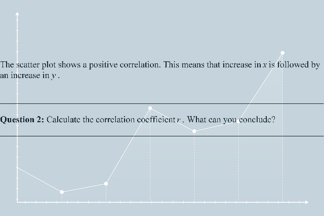
Question 1: Construct a scatter plot for the data. Do the data appear to have a positive linear correlation, a negative correlation, or no linear correlation? Explain.
Question 2: Calculate the correlation coefficient \(r\). What can you conclude?
Question 3: Test the level of significance of the correlation coefficient. Use \(\alpha =0.05\)
Question 4: Find the equation of the regression line for the data. Include the regression line in the scatter plot.
Question 5: Use the regression line to predict the personal outlays when the personal income is 5.3 trillion dollars.
Question 6: Find the coefficient of determination and interpret the results.
Question 7: Find the standard error of the estimate \({{s}_{e}}\) and interpret the results.
Question 8: Construct a 95% prediction interval for personal outlays when personal income is 6.4 trillion dollars. Interpret the results.
Question 9: The equation used to predict sunflower yield (in pounds) is
\[\hat{y}=1257-1.34{{x}_{1}}+1.41{{x}_{2}}\]
where \({{x}_{1}}\) is the number of acres planted (in thousands) and \({{x}_{2}}\) is the number of acres harvested (in thousands). Use the regression equation to predict the y-values for the given values of the independent variable listed below. Then determine which variable has a greater influence on the value of \(y\)
(a) \({{x}_{1}}=2103,\text{ }{{x}_{2}}=2037\) (b) \({{x}_{1}}=3387,\text{ }{{x}_{2}}=3009\)
(c) \({{x}_{1}}=2185,\text{ }{{x}_{2}}=1980\) (d) \({{x}_{1}}=3485,\text{ }{{x}_{2}}=3404\)
Question 11: A legal researcher is studying the age distribution of juries by comparing them with the overall age distribution of available jurors. The researcher claims that the jury distribution is different from the overall distribution; that is, there is a noticeable age bias in jury selection in this area. The table shows the number of jurors at a county court in one year and the percent of persons residing in that county, by age. Use the population distribution to find the expected juror frequencies. Test the researcher’s claim at \(\alpha =0.01\).
|
21-29 |
30-39 |
40-49 |
50-59 |
60 and above | |
|
Jury |
45 |
128 |
244 |
224 |
359 |
|
Population |
20.50% |
21.70% |
18.10% |
17.30% |
22.40% |
Question 14: The table shows the age distribution of a random sample of fatally injured male and female passenger vehicle drivers whose blood alcohol content was at least 0.08 in a recent year. Use \(\alpha =0.05\).
|
Gender |
16-20 |
21-30 |
31-40 |
41-50 |
51-60 |
61+ |
|
Male |
155 |
280 |
265 |
225 |
155 |
50 |
|
Female |
60 |
145 |
145 |
130 |
65 |
15 |
In exercises 20 and 21, find the critical F-value for a right-tailed test using the indicated level of significance \(\alpha \) and degrees of freedom d.f.N and d.f.D
Question 20: \(\alpha =0.05\), d.f.N = 6, d.f.D = 50
Question 21: \(\alpha =0.10\), d.f.N = 5, d.f.D = 12
Question 26: A steel pipe fittings company claims that the yield strength of its nontempered couplings is more variable than that of its tempered couplings. A random sample of nine tempered couplings has a standard deviation of 1.31 megapascals, and a similar sample of nine nontempered couplings has a standard deviation of 25.4 megapascals. From past data, it is known that the company’s production process results in normally distributed yield strengths. Test the company’s claim at \(\alpha =0.05\)
Deliverable: Word Document
 and pdf


![[Solved] Your final report needs to be compiled with regard to - #80181 Statistics](/images/projects/project-80181/statistics-1.jpg)

