Question: When a variable is difficult to measure it is common to use easier-to-measure variables that are related to the variable of interest. An example involving bears is the weight of a bear. For reasons of safety the bears are anesthetized in the wild for measuring. It is relatively easy to measure various lengths using a tape measure and the age of a bear, but it is difficult to find the weight of a bear because it must be lifted. Can the weight of a bear be predicted from another measurement? The weight (in pounds) and chest girth of 75 anesthetized bears are recorded. Let y = weight, x = chest girth. The linear regression model Y = β₀ + β₁x was estimated using the least squares method. Use the Minitab output on pages 5 and 6 to answer the following questions.

(a) Write down the least squares equation to the linear regression model Y = β₀+ β₁x. (1 mark)

(b) What is the predicted weight of a bear if the bear has a chest girth of 34 inches? (2 marks)

(c) What is the value of the coefficient of determination? What does this value tell you about the fit of the model? What is the precise interpretation of the coefficient of determination? (2 marks)

(d) Interpret the estimate of the slope coefficient β₁. (2 marks)

(e) Interpret the estimate of the intercept coefficient β₀. (2 marks)

(f) Suppose a bear is found to have a chest girth of 34 inches. Estimate the weight of this bear with 95% confidence. (2 marks)

(g) Suppose another bear is found to have a chest girth of 25 inches. Would the 95% interval estimate for the weight of this bear be narrower than the interval found in part (f)? Explain. (3 marks)

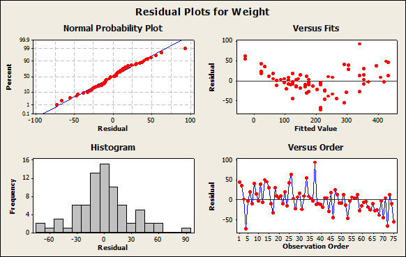
(h) Use the residual analysis to check whether the linearity, equal variance, independence and normality requirements are satisfied. (4 marks)