Client
Statistician	A	B	C
1	150	210	270
2	170	230	220
3	180	230	225
4	160	240	230

a. Formulate and solve a linear programming model for this problem.

b. Suppose that the time it takes statistician 4 to complete the job for client A is increased

from 160 to 165 hours. What effect will this change have on the solution?

c. Suppose that the time it takes statistician 4 to complete the job for client A is decreased to 140 hours. What effect will this change have on the solution?

d. Suppose that the time it takes statistician 3 to complete the job for client B increased

to 250 hours. What effect will this change have on the solution?

Solution:

(a) We have the decision variables \({{x}_{ij}}\), which is 0 or 1 depending on if the statistician i is assigned to the client j.

We need to solve the following problem:

\[\begin{aligned} & \text{Minimize}\,\,\text{ }\sum{{{C}_{ij}}{{X}_{ij}}} \\

& s.t. \\

& \,\,\,\,\,\,\,\,\,\,\,\,\,\,\,\,\,\,\,\,\,\,\,\,{{x}_{11}}+{{x}_{12}}+{{x}_{13}}\le 1 \\

& \,\,\,\,\,\,\,\,\,\,\,\,\,\,\,\,\,\,\,\,\,\,\,\,{{x}_{21}}+{{x}_{22}}+{{x}_{23}}\le 1 \\

& \,\,\,\,\,\,\,\,\,\,\,\,\,\,\,\,\,\,\,\,\,\,\,\,{{x}_{31}}+{{x}_{32}}+{{x}_{33}}\le 1 \\

& \,\,\,\,\,\,\,\,\,\,\,\,\,\,\,\,\,\,\,\,\,\,\,\,{{x}_{41}}+{{x}_{42}}+{{x}_{43}}\le 1 \\

& \,\,\,\,\,\,\,\,\,\,\,\,\,\,\,\,\,\,\,\,\,\,\,\,{{x}_{11}}+{{x}_{21}}+{{x}_{31}}+{{x}_{41}}=1 \\

& \,\,\,\,\,\,\,\,\,\,\,\,\,\,\,\,\,\,\,\,\,\,\,\,{{x}_{12}}+{{x}_{22}}+{{x}_{32}}+{{x}_{42}}=1 \\

& \,\,\,\,\,\,\,\,\,\,\,\,\,\,\,\,\,\,\,\,\,\,\,\,{{x}_{13}}+{{x}_{23}}+{{x}_{33}}+{{x}_{43}}=1 \\

& \,\,\,\,\,\,\,\,\,\,\,\,\,\,\,\,\,\,\,\,\,\,\,\,{{x}_{ij}}\in \{0,1\} \\

\end{aligned}\]

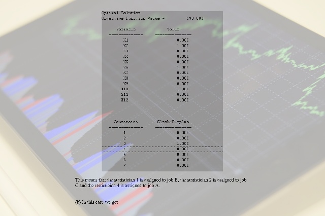
Using the Management Scientist we get the following output:

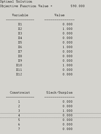
This means that the statistician 1 is assigned to job B, the statistician 2 is assigned to job C and the statistician 4 is assigned to job A.

(b) In this case we get

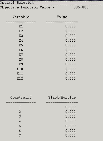
As we can see, the assignment doesn’t change, only the total time increases in 5 hours

(c) In this case we obtain:

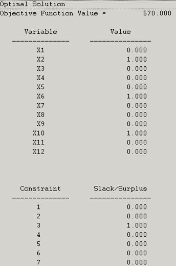
The again, the assignment doesn’t change, only the total time is reduced in 20 hours

(d) The new output is

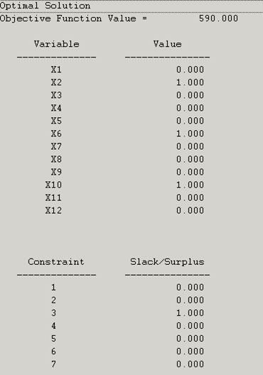
The assignment again doesn’t change.

Problem 2:

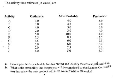
Solution: We have the following schedule:

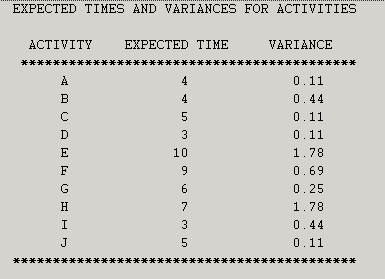
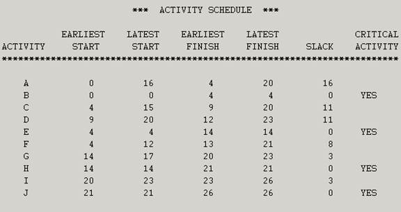
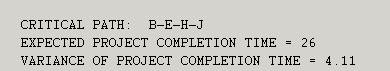
This means that the critical path is B-E-H-J. The expected completion time is 26 weeks.

(b) Let X be the completion time, we need to compute

\[\Pr \left( X<25 \right)=\Pr \left( \frac{X-26}{\sqrt{4.11}}<\frac{25-26}{\sqrt{4.11}} \right)=\Pr \left( Z<-0.49326 \right)=0.310913\]

Also,

\[\Pr \left( X<30 \right)=\Pr \left( \frac{X-26}{\sqrt{4.11}}<\frac{30-26}{\sqrt{4.11}} \right)=\Pr \left( Z< \right)=0.975755\]

\

Problem 3:

• For the EOQ we have:

Inventory	Economic Order Quantity Model
Data
Demand rate, D	800
Setup cost, S	150
Holding cost, H	3
Unit Price, P
Daily demand rate	3.2
Lead time in days
Results
Optimal Order Quantity, Q*	282.842712
Maximum Inventory	282.842712
Average Inventory	141.421356
Number of Setups	2.82842712
Holding cost	$424.26
Setup cost	$424.26
Unit costs	-
Total cost, Tc	$848.53
Reorder Point	-

• For the backorder model:

Inventory	EOQ with shortages
Data
Demand rate, D	800
Setup cost, S	150
Holding cost, H	3
Shortage cost	20
Unit Price, P
Results
Optimal Order Quantity, Q*	303.315
Maximum Inventory	263.7522
Average Inventory	114.6749
Number of Setups	2.637522
Maximum Backorders	39.56283
Holding cost	344.0246
Setup cost	395.6283
Backorder cost	51.60369
Unit costs
Total cost	791.2566

This means that the backorder model is cheaper. The difference is $848.54 - $791.2566 = $57.2834.

• In this case, the percentage of units backordered is

\[\frac{39.56283}{114.6749}\times 100=34.5%\]

which is too high. The maximum time a customer will wait for a backordered item is

\[t=\frac{S}{d}=\frac{39.56283}{3.2}=12.36\text{ days}\]

which is within the manager’s limits.