In this tutorial, we are going to be covering the topic of Non-parametric tests . See below a list of relevant sample problems, with step by step solutions.
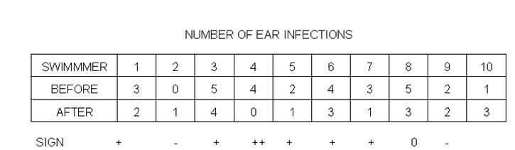
Question 1: A medical researcher believes the number of ear infections in swimmers can be reduced if the swimmers use ear plugs. A sample of ten people was selected, and the number of ear infections for a four-month period was recorded. During the first two months, the swimmers did not use the ear plugs; during the second two months, they did. At the beginning of the second two-month period, each swimmer was examined to make sure that no infections were present. The data are shown below. At \(\alpha = 0.05\), can the researcher conclude that using ear plugs effects the number of ear infections?
Solution: We need to test the hypotheses
\[\begin{aligned} & {{H}_{0}}:\text{ ear infections are the same with or without the ear plugs} \\ &{{H}_{A}}:\text{ swimmers get less ear infections with ear plugs} \\ \end{aligned}\]
We use a Sign-Test. We use Statdisk to get the following output:
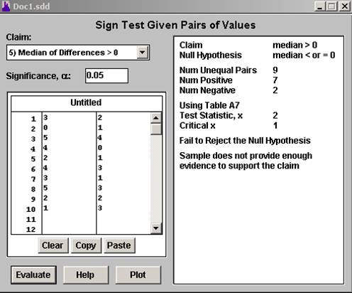
The \(x\) statistics is equal to 2 (the less frequent number of signs). The critical value is 1. Since \(x\) is not less than or equal to the critical value, we fail to reject the null hypothesis. This means that we don't have enough evidence to support the claim that the number of ear infections in swimmers can be reduced if the swimmers use ear plugs.
Question 2: Research indicates that people who volunteer to participate in research studies tend to have higher intelligence than nonvolunteers. To test this phenomenon, a researcher obtains a sample of 200 high school students. The students are given a description of a psychological research study and asked whether they would volunteer to participate. The researcher also obtains an IQ score for each student and classifies the students into high, medium, and low IQ groups. Do the following data indicate a significant relationship between IQ and volunteering? Test at the .05 level of significance.
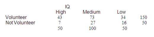
Solution: The following table shows the corresponding contingency table:
|
Observed |
High |
Medium |
Low |
Total |
|
Volunteer |
43 |
73 |
34 |
150 |
|
Not Volunteer |
7 |
27 |
16 |
50 |
|
Total |
50 |
100 |
50 |
200 |
We are interested in testing the following null and alternative hypotheses:
\[\begin{aligned}{{H}_{0}}:\,\,\, \text{Volunteer Status}\text{ and }\text {IQ}\text{ are independent} \\ {{H}_{A}}:\,\,\,\text{Volunteer Status}\text{ and }\text {IQ}\text{ are NOT independent} \\ \end{aligned}\]
From the table above we compute the table with the expected values
|
Expected |
High |
Medium |
Low |
|
Volunteer |
37.5 |
75 |
37.5 |
|
Not Volunteer |
12.5 |
25 |
12.5 |
The way those expected frequencies are calculated is shown below:
\[{E}_{{1},{1}}= \frac{ {R}_{1} \times {C}_{1} }{T}= \frac{{150} \times {50}}{{200}}={37.5},\,\,\,\, {E}_{{1},{2}}= \frac{ {R}_{1} \times {C}_{2} }{T}= \frac{{150} \times {100}}{{200}}={75},\,\,\,\, {E}_{{1},{3}}= \frac{ {R}_{1} \times {C}_{3} }{T}= \frac{{150} \times {50}}{{200}}={37.5}\]
\[,\,\,\,\, {E}_{{2},{1}}= \frac{ {R}_{2} \times {C}_{1} }{T}= \frac{{50} \times {50}}{{200}}={12.5},\,\,\,\, {E}_{{2},{2}}= \frac{ {R}_{2} \times {C}_{2} }{T}= \frac{{50} \times {100}}{{200}}={25},\,\,\,\, {E}_{{2},{3}}= \frac{ {R}_{2} \times {C}_{3} }{T}= \frac{{50} \times {50}}{{200}}={12.5}\]
Finally, we use the formula \(\frac{{{\left( O-E \right)}^{2}}}{E}\) to get
|
(fo - fe)²/fe |
High |
Medium |
Low |
|
Volunteer |
0.8067 |
0.0533 |
0.3267 |
|
Not Volunteer |
2.42 |
0.16 |
0.98 |
The calculations required are shown below:
\[\frac{ {\left( {43}-{37.5} \right)}^{2} }{{37.5}} ={0.8067},\,\,\,\, \frac{ {\left( {73}-{75} \right)}^{2} }{{75}} ={0.0533},\,\,\,\, \frac{ {\left( {34}-{37.5} \right)}^{2} }{{37.5}} ={0.3267},\,\,\,\, \frac{ {\left( {7}-{12.5} \right)}^{2} }{{12.5}} ={2.42}\]
\[,\,\,\,\, \frac{ {\left( {27}-{25} \right)}^{2} }{{25}} ={0.16},\,\,\,\, \frac{ {\left( {16}-{12.5} \right)}^{2} }{{12.5}} ={0.98}\]
Hence, the value of Chi-Square statistics is
\[{{\chi }^{2}}=\sum{\frac{{{\left( {{O}_{ij}}-{{E}_{ij}} \right)}^{2}}}{{{E}_{ij}}}}={0.8067} + {0.0533} + {0.3267} + {2.42} + {0.16} + {0.98} = 4.747\]
The critical Chi-Square value for \(\alpha =0.05\) and \(\left( 3-1 \right)\times \left( 2-1 \right)=2\) degrees of freedom is \(\chi _{C}^{2}= {5.991}\). Since \({{\chi }^{2}}=\sum{\frac{{{\left( {{O}_{ij}}-{{E}_{ij}} \right)}^{2}}}{{{E}_{ij}}}}= {4.747}\) < \(\chi _{C}^{2}= {5.991}\), then we fail to reject the null hypothesis, which means that we don't have enough evidence to reject the null hypothesis of independence.
Question 3: Listed below are the numbers of years that U.S. presidents, popes since 1690 and British monarchs lived after they were inaugurated, elected, or coronated. As of the writing, the last president is Gerald Ford and the last pope is John Paul II. The times are based on data from Computer interactive Data Analysis, by Lunn and McNeil, John Wiley & Son. Use a 0.05 significance level to test the claim that the 2 samples of longevity data from popes and monarchs are from populations with the same median.
Presidents
10 29 26 28 15 23 17 25 0 20 4 1 24 16 12 4 10 17 16 0 7 24 12 4
18 21 11 2 9 36 12 28 3 16 9 25 23 32
Popes
2 9 21 3 6 10 18 11 6 25 23 6 2 15 32 25 11 8 17 19 5 15 0 26
Monarchs 17 6 13 12 13 33 59 10 7 63 9 25 36 15
Solution: We need to use a Wilcoxon test in order to assess the claim that the 2 samples are from populations with the same median. The following results are obtained:
|
Wilcoxon - Mann/Whitney Test |
||||
|
n |
sum of ranks |
|||
|
24 |
416 |
Popes |
||
|
14 |
325 |
Monarchs |
||
|
38 |
741 |
total |
||
|
468.00 |
expected value |
|||
|
33.00 |
standard deviation |
|||
|
-1.56 |
z, corrected for ties |
|||
|
.1186 |
p-value (two-tailed) |
|||
|
No. |
Label |
Data |
Rank |
|
|
1 |
Popes |
2 |
2.5 |
|
|
2 |
Popes |
9 |
12.5 |
|
|
3 |
Popes |
21 |
28 |
|
|
4 |
Popes |
3 |
4 |
|
|
5 |
Popes |
6 |
7.5 |
|
|
6 |
Popes |
10 |
14.5 |
|
|
7 |
Popes |
18 |
26 |
|
|
8 |
Popes |
11 |
16.5 |
|
|
9 |
Popes |
6 |
7.5 |
|
|
10 |
Popes |
25 |
31 |
|
|
11 |
Popes |
23 |
29 |
|
|
12 |
Popes |
6 |
7.5 |
|
|
13 |
Popes |
2 |
2.5 |
|
|
14 |
Popes |
15 |
22 |
|
|
15 |
Popes |
32 |
34 |
|
|
16 |
Popes |
25 |
31 |
|
|
17 |
Popes |
11 |
16.5 |
|
|
18 |
Popes |
8 |
11 |
|
|
19 |
Popes |
17 |
24.5 |
|
|
20 |
Popes |
19 |
27 |
|
|
21 |
Popes |
5 |
5 |
|
|
22 |
Popes |
15 |
22 |
|
|
23 |
Popes |
0 |
1 |
|
|
24 |
Popes |
26 |
33 |
|
|
25 |
Monarchs |
17 |
24.5 |
|
|
26 |
Monarchs |
6 |
7.5 |
|
|
27 |
Monarchs |
13 |
19.5 |
|
|
28 |
Monarchs |
12 |
18 |
|
|
29 |
Monarchs |
13 |
19.5 |
|
|
30 |
Monarchs |
33 |
35 |
|
|
31 |
Monarchs |
59 |
37 |
|
|
32 |
Monarchs |
10 |
14.5 |
|
|
33 |
Monarchs |
7 |
10 |
|
|
34 |
Monarchs |
63 |
38 |
|
|
35 |
Monarchs |
9 |
12.5 |
|
|
36 |
Monarchs |
25 |
31 |
|
|
37 |
Monarchs |
36 |
36 |
|
|
38 |
Monarchs |
15 |
22 |
|
Since we are comparing two independent groups (Popes & Monarchs), we can use Wilcoxon Rank Sum Test.
The null hypothesis tested is
H0: The two samples are from populations with the same median.
The alternative hypothesis is
H1: The two samples are from populations with the different median.
Significance level = 0.05
Test statistic: The observed values from the pooled sample results are ranked from smallest to largest. After the rankings are obtained, the samples are separated, and the sum of the rankings is calculated for each.
The test statistic used is
\[Z=\frac{{{T}_{A}}-\frac{{{n}_{2}}\left( {{n}_{1}}+{{n}_{2}}+1 \right)}{2}}{\sqrt{\frac{{{n}_{1}}{{n}_{2}}\left( {{n}_{1}}+{{n}_{2}}+1 \right)}{12}}}\]
,
where T A is the sum of ranks of the smaller sample. Here n 1 = 24, n 2 = 14, T A = 416.
Therefore,\[Z=\frac{416-\frac{24\left( 14+24+1 \right)}{2}}{\sqrt{\frac{14*24\left( 14+24+1 \right)}{12}}}=-1.57\]
Rejection criteria: Reject the null hypothesis, if the absolute value of test statistic is greater than the critical value at the 0.05 significance level.
Lower critical value = -1.96
Upper critical value = 1.96
Conclusion: Fails to reject the null hypothesis, since the absolute value of test statistic is less than the critical value. The sample does not provide enough evidence to reject the claim that the two samples are from populations with the same median.
In case you have any suggestion, or if you would like to report a broken solver/calculator, please do not hesitate to contact us .