Chi-Square Test for Goodness of Fit

More about the Chi-Square test for goodness of fit calculator so that you can interpret in a better way the results delivered by this calculator

What is a chi-square Calculator for goodness-of-fit?

A Chi-Square for goodness of fit test calculator is a test used to assess whether the observed data can be claimed to reasonably fit the expected data.

Sometimes, a Chi-Square test for goodness of fit is referred as a test for multinomial experiments, because there is a fixed number of N categories, and each of the outcomes of the experiment falls in exactly one of those categories.

Then, based on sample information, the test uses a Chi-Square statistic to assess if the expected proportions for all categories reasonably fit the sample data.

What are the main properties of the Chi-Square distribution?

The main properties of a one sample Chi-Square test for goodness of fit are:

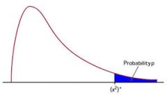
• The distribution of the test statistic is the Chi-Square distribution, with n-1 degrees of freedom, where n is the number of categories


• The Chi-Square distribution is one of the most important distributions in statistics, together with the normal distribution and the F-distribution


• The Chi-Square test of goodness of fit is right-tailed

Chi-Square goodness of fit formula

The formula for a Chi-Square statistic calculation is given by

\[\chi^2 = \sum_{i=1}^n \frac{(O_i-E_i)^2 }{E_i} \]

One of the most common uses for this test is to assess whether a sample come from a population with a specific population (this is, for example, using this test we can assess if a sample comes from a normally distributed population or not).

Goodness of fit calculator example

Question: A researcher wants to investigate the colors of the candies that come in a box. There is the claim that all the colors are equally likely. The possible colors are red, green and blue, and the sample found 55 red candies, 43 green, and 38 blue. Can you disprove the claim that all colors are equally likely?

Solution:

We need to conduct a Chi-Square test of Goodness of Fit. The following information has been provided:

Categories	Observed	Expected Proportions
A	55	1/3
B	34	1/3
C	34	1/3

Now, we need to compute the expected values and squared distances in order to find the Chi-Square statistic. The following is obtained:

Categories	Observed	Expected	(fo-fe)2/fe
A	55	\(123 \times \frac{1}{3} = 41\)	\(\displaystyle\frac{ \left( 55-41\right)^2}{ 41} = 4.78\)
B	34	\(123 \times \frac{1}{3} = 41\)	\(\displaystyle\frac{ \left( 34-41\right)^2}{ 41} = 1.195\)
C	34	\(123 \times \frac{1}{3} = 41\)	\(\displaystyle\frac{ \left( 34-41\right)^2}{ 41} = 1.195\)
Sum =	123	123	7.171

(1) Null and Alternative Hypotheses

The following null and alternative hypotheses need to be tested:

\(H_0: p_1 = \frac{1}{3}, p_2 = \frac{1}{3}, p_3 = \frac{1}{3}\)

\(H_a\): Some of the population proportions differ from the values stated in the null hypothesis

This corresponds to a Chi-Square test for Goodness of Fit.

(2) Rejection Region

Based on the information provided, the significance level is \(\alpha = 0.03\), the number of degrees of freedom is \(df = 3 - 1 = 2\), so then the rejection region for this test is \(R = \{\chi^2: \chi^2 > 7.013\}\).

(3) Test Statistics

The Chi-Squared statistic is computed as follows:

\[ \begin{array}{ccl} \chi^2 & = & \displaystyle \sum_{i=1}^n {\frac{(O_i-E_i)^2}{E_i}} \\\\ \\\\ & = & \displaystyle 4.78+1.195+1.195 \\\\ \\\\ & = & 7.171 \end{array}\]

(4) Decision about the null hypothesis

Since it is observed that \(\chi^2 = 7.171 > \chi_c^2 = 7.013\), it is then concluded that the null hypothesis is rejected.

(5) Conclusion

It is concluded that the null hypothesis Ho is rejected. Therefore, there is not enough evidence to claim that some of the population proportions differ from those stated in the null hypothesis, at the \(\alpha = 0.03\) significance level.