(15 marks) Download the Excel file A1Q1.xlsx from Moodle. The spreadsheet contains 30 randomly generated
- (15 marks) Download the Excel file A1Q1.xlsx from Moodle. The spreadsheet contains 30 randomly generated numbers.
- Use the descriptive statistics feature in Excel to calculate the descriptive statistic. Attach the Excel output. (3 marks)
- Construct a 95-percent confidence interval for the population variance and the population mean. (4 marks)
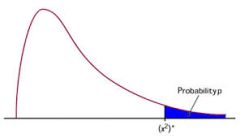
- At the 90-percent level of confidence, test whether the population variance equals 25. Carefully state the null and alternative hypotheses, calculate the appropriate test statistic, state the appropriate critical value and explain your decision. (4 marks)
- At the 99-percent level of confidence, test whether the population mean equals zero. Carefully state the null and alternative hypotheses, calculate the appropriate test statistic, state the appropriate critical value and explain your decision. (4 marks)
2. (2 marks each = 22 marks) Write the following summations in expanded form
- \(\sum\limits_{i=1}^{5}{3k}\)
- \(\frac{1}{4}\sum\limits_{m=1}^{4}{{{x}_{m}}}\)
- \(\sum\limits_{j=4}^{n}{\frac{j}{j+1}}\)
- \(\sum\limits_{i=1}^{4}{\frac{{{\left( {{O}_{i}}-{{E}_{i}} \right)}^{2}}}{{{E}_{i}}}}\)
- \(\sum\limits_{j=3}^{7}{{{3}^{j-1}}}\)
- \(\frac{1}{5}\sum\limits_{k=1}^{5}{{{x}_{k}}}\)
- \[2\sum\limits_{t=2}^{m}{\frac{t-1}{t+1}}\]
- \(\frac{1}{n-1}\sum\limits_{i=1}^{n}{{{\left( {{x}_{i}}-\bar{x} \right)}^{2}}}\)
- \(\sum\limits_{i=1}^{5}{2{{l}^{2}}}\)
- \(\sum\limits_{k=1}^{3}{{{5}^{k+1}}}\)
- \(\sum\limits_{i=1}^{k+1}{\frac{3\left( i-2 \right)}{i+2}}\)
3. Use the provided data to answer the following questions.
| \[{{X}_{i}}\] | \[{{Y}_{i}}\] | \[X_{i}^{2}\] | \[{{X}_{i}}{{Y}_{i}}\] | \[{{\hat{Y}}_{i}}\] | \[{{e}_{i}}\] | \[{{e}_{i}}^{2}\] | \[{{Y}_{i}}-\bar{Y}\] | \[{{\left( {{Y}_{i}}-\bar{Y} \right)}^{2}}\] | \[{{\hat{Y}}_{i}}-\bar{Y}\] | \[{{\left( {{{\hat{Y}}}_{i}}-\bar{Y} \right)}^{2}}\] | |
| 7 | 2 | ||||||||||
| 4 | 4 | ||||||||||
| 6 | 2 | ||||||||||
| 2 | 5 | ||||||||||
| 1 | 7 | ||||||||||
| 1 | 6 | ||||||||||
| 3 | 5 | ||||||||||
| Sum = | 24 | 31 | 116 | 80 | 1.2203 | 21.7143 | 20.4939 |
- Fill in the above table.
- Calculate \(\bar{X}\)
- Calculate \(\bar{Y}\)
- Calculate \(\operatorname{cov}(X, Y)\). (2 marks)
- Calculate \(\operatorname{var}(X)\). (2 marks)
- Calculate \({{\hat{\beta }}_{1}}\)
- Calculate \({{\hat{\beta }}_{0}}\)
- Calculate RSS
- Calculate ESS. (1 mark)
- Calculate TSS. (1 mark)
- Calculate \(R^{2}\). (1 mark)
- Calculate \(r\). (1 mark)
- Calculate MSE. (1 mark)
- Calculate MSR. (1 mark)
- Calculate \(s\). (1 mark)
4. A marketing manager wants to establish the relationship between the number of cereal boxes sold, \(B\), and the shelf space in square feet devoted to them, $S$. This relationship is assumed to be linear of the form shown below:
\(B_{i}=\beta_{0}+\beta_{1} S_{i}+\varepsilon_{i} \text {, for } i=1, \ldots, n\)
- Predict and justify the sign that you would expect for \(\beta_{1}\). (2 marks)
- Download the Excel file A1Q4.xlsx from Moodle. The spreadsheet contains weekly sales of cereal boxes and the shelf space in square feet devoted to them for 14 urban grocery stores. Estimate the regression in Excel, attach your Excel output and write down the estimated regression equation. (4 marks)
- Interpret the estimated coefficients. (2 marks)
- Calculate the residuals and plot them against the independent variable. Attach your Excel graph. (4 marks)
- Delete the \(8^{\text {th }}, 11^{\text {th }}, 12^{\text {th }}\) and \(13^{\text {th }}\) observations and re-estimate the regression in Excel. Attach your Excel output and write down the new estimated regression equation. (4 marks)
- Graph the estimated regression equations lines from (b) and (e). Do they intersect and, if so, at what point? (3 marks)
- Compare the estimated coefficients in (b) and (e). Briefly explain why they differ? (2 marks)
- Compare the \(R^{2}\) coefficients in (b) and (e). Which one is better and why? (2 marks)
5. A farmer wants to establish the relationship between the per-acre yield of corn, \(Y\) (measured in bushels per acre), and the average July temperature in Manitoba, \(X\) (measured in degrees Fahrenheit), using information from the past eight years. Preliminary analysis of the sample data produces the following information:
\(\sum Y_{i}=848 \quad \sum X_{i}=736 \quad \sum Y_{i}^{2}=91334 \quad \sum X_{i}^{2}=67852\)
\(\sum X_{i} Y_{i}=78429 \quad \sum e_{i}^{2}=227.65 \quad \sum\left(X_{i}-\bar{X}\right)\left(Y_{i}-\bar{Y}\right)=413\)
Use the above sample information to answer all the following questions. Show explicitly all formulas and calculations.
- Calculate the estimated intercept coefficient, \(\beta_{0}\), and slope coefficient, \(\beta_{1}\). (4 marks)
- Write down the estimated regression equation and interpret the value of the slope coefficient. (4 marks)
- Calculate the estimated error variance, \(\hat{\sigma}^{2}\). (2 marks)
- Calculate the coefficient of determination, \(R^{2}\). Briefly explain what it means. (4 marks)
Deliverable: Word Document


![[All Steps] (50 marks) Download the Excel file A2Q1.xlsx from [All Steps] (50 marks) Download the Excel](/images/solutions/MC-solution-library-82512.jpg)


![[Step-by-Step] Food Prices Governments throughout the world are concerned [Step-by-Step] Food Prices Governments throughout the world](/images/solutions/MC-solution-library-82515.jpg)
![[Solution Library] A1: Assignment General mental ability (GMA) [Solution Library] A1: Assignment General mental ability](/images/solutions/MC-solution-library-82516.jpg)
