Empirical Rule Calculator
Instructions: This Empirical Rule calculator with steps will show you how to use the Empirical Rule to compute some normal probabilities. Please type the population mean and population standard deviation, and provide details about the event you want to compute the probability for. Observe that not all events can have their probability computed with these technique. For a general normal probability calculator, please check here .
More About the Empirical Rule
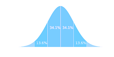
The Empirical Rule states that the area under the normal distribution that is within one standard deviation of the mean is approximately 0.68, the area within two standard deviations of the mean is approximately 0.95, and the area within three standard deviations of the mean is approximately 0.997.
It needs to be observed that these are approximations only. Using the exact normal distribution tables, for example, the area within two standard deviations of the mean is more like 0.954500, instead of 0.95, although 0.95 is a simpler to remember number.
Using this Empirical Rule only a handful number probabilities can be computed. For the general case, use this normal probability calculator .
Is there an Empirical Rule formula?
More than a formula, the empirical rule tells an approximation of the percentage of distribution contained by the intervals \((\mu - \sigma, \mu + \sigma)\), \((\mu - 2\sigma, \mu + 2 \sigma)\) and \((\mu + 3\sigma, \mu + 3\sigma)\)
Relationship between Chebyshev's theorem and the Empirical Rule
Notice that the empirical rule is applicable only to normal distributions. For the case of general, non-normal distributions, you should use instead our Chebyshev's inequality calculator , or even Markov's inequality for non-negative random variables.
Observe that sometimes the empirical rule is referred as the 68-95-99.7 Rule Calculator, because of the probabilities associated with the rule.
Summarizing
The empirical rule is an approximate that describes very accurately the behavior of the normal distribution, in terms of the area under the curve within a certain number of standard deviations from the mean.
Indeed, the empirical rule states that
- Approximately 68% of the normal distribution is within one standard deviation of the mean.
- Approximately 95% of the normal distribution is within two standard deviations of the mean.
- Approximately 99.7% of the normal distribution is within three standard deviations of the mean.
Notice the term "approximately" because those are not exact. If you use Excel you will find using the formula that the probability within 2 standard deviations is more like 0.9544997 or 95.44997% (depending on how many decimals you use) , but the approximation of 95% works fairly well for many applications.
If you need to depict the graphical situation, you can use this normal probability grapher .
Example of Using the Empirical Rule
Question : Assume that \(X\) has a distribution with mean \(\mu = 45\) and standard deviation \(\sigma = 12\). Using the empirical rule, compute the probability that \(X\) is on the interval (21, 45).
Solution:
The following are the population mean \((\mu)\) and population standard deviation \((\sigma)\) provided:
| Population Mean \((\mu)\) = | \(45\) |
| Population Standard Deviation \((\sigma)\) = | \(12\) |
Preliminary calculations
The Empirical Rule tells us about the approximate probability that is found within a certain number of standard deviations from the population mean.
• First, the Empirical Rule says that the probability within 1 standard deviation from the mean is approximately 68%.
This means that:
\[ \Pr(\mu - \sigma \le X \le \mu + \sigma) \approx 0.68 \]In this case, we have that:
\[ \mu - \sigma = 45- 12 = 33\]\[ \mu + \sigma = 45+ 12 = 57\]so then
\[ \Pr(33\le X \le 57) \approx 0.68 \]Then, since the probability inside of the interval \(33, 57\) is 0.68, then using the Law of Complement, the probability OUTSIDE of \(33, 57\) is 1 - 0.68 = 0.32. Also, since the normal distribution is symmetric, then we also conclude that half of that probability (0.32/2 = 0.16) goes to each of the two tails. This means that
\[ \Pr(X \le 33) \approx 0.16 \]\[ \Pr(X \le 57) \approx 1 - 0.16 = 0.84\]• Similarly, the Empirical Rule says that the probability within 2 standard deviations from the mean is approximately 95%. This means that:
\[ \Pr(\mu - 2 \sigma \le X \le \mu + 2\sigma) \approx 0.95 \]In this case, we have that:
\[ \mu - 2\sigma = 45- 2\times 12 = 21 \]\[ \mu + 2 \sigma = 45+ 2\times 12 = 69 \]so then
\[ \Pr(21 \le X \le 69) \approx 0.95 \]Then, since the probability inside of the interval \(21, 69\) is 0.95, then using the Law of Complement, the probability OUTSIDE of \(21, 69\) is 1 - 0.95 = 0.05. Also, since the normal distribution is symmetric, then we also conclude that half of that probability (0.05/2 = 0.025) goes to each of the two tails. This means that
\[ \Pr(X \le 21) \approx 0.025 \]\[ \Pr(X \le 69) \approx 1 - 0.025 = 0.975\]• Finally, the Empirical Rule says that the probability within 2 standard deviations from the mean is approximately 99.7%. This means that:
\[ \Pr(\mu - 3 \sigma \le X \le \mu + 3\sigma) \approx 0.997 \]In this case, we have that:
\[ \mu - 3\sigma = 45- 3\times 12 = 9 \]\[ \mu + 3\sigma = 45+ 3\times 12 = 81 \]so then
\[ \Pr(9 \le X \le 69) \approx 0.997 \]Then, since the probability inside of the interval \(9, 81\) is 0.997, then using the Law of Complement, the probability OUTSIDE of \(9, 81\) is 1 - 0.997 = 0.003. Also, since the normal distribution is symmetric, then we also conclude that half of that probability (0.003/2 = 0.0015) goes to each of the two tails. This means that
\[ \Pr(X \le 9) \approx 0.0015 \]\[ \Pr(X \le 81) \approx 1 - 0.0015 = 0.9985\]Summary of what we know
Summarizing, these are the probabilities that we know approximately, based on the Empirical Rule:
\( \Pr(X \le 9) \approx 0.0015\)\( \Pr(X \le 21) \approx 0.025\)
\( \Pr(X \le 33) \approx 0.16\)
\( \Pr(X \le 69) \approx 0.975 \)
\( \Pr(X \le 81) \approx 0.9985\)
Calculation of the probability
Now, we need to break down the probability we need to compute into two probabilities we know from the list we created above. Indeed, we get that:
\[ \Pr(21 \le X \le 45) = \Pr(X \le 45) - \Pr(X \le 21)\]\[ \approx 0.5 - 0.025 = 0.475\]which concludes the calculation.

