Statistics Tutorials

ANOVA Tutorial

In this week's tutorial, we are going to be covering the topic of Analysis of Variance . See below a list of relevant sample problems, with step sy step solutions.

We hope you will find them useful. We share full tutorials, tips and hints, with the members of our community. Please do not hesitate to contact us if you any questions.

Sample ANOVA problems

Question 1: An analysis of variance was used to evaluate the mean differences from a repeated-measures research study. The results were reported as F(3,24)=6.40.

a. How many treatment conditions were compared in the study?

b. How many individuals participated in the study?

Solution: (a) There were 3+1 = 4 treatment conditions.

(b) The total number of individuals is 3 + 24 + 1 = 28.

Question 2: The following data represent the results from an independent-measures study comparing three treatments.

a. Compute SS for the set of 3 treatment means. (Use the three means as a set of n = 3 scores and compute SS.)

b. Using the result from part a, compute n (SSmeans). Note that this value is equal to SS between (see Equation 13.6).

c. Now, compute SSbetween with the computational formula using the T values (Equation 13.7). You should obtain the same result as in part b.

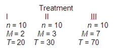
Solution: (a) We get that \(\bar{M}=\frac{2+3+7}{3}=4\)

which means that

\[S{{S}_{Means}}={{\left( 2-4 \right)}^{2}}+{{\left( 3-4 \right)}^{2}}+{{\left( 7-4 \right)}^{2}}=4+1+9=14\]

(b) This implies that \(n*S{{S}_{Means}}=10\times 14=140\).

\[S{{S}_{Between}}=\frac{{{20}^{2}}}{10}+\frac{{{30}^{2}}}{10}+\frac{{{70}^{2}}}{10}-\frac{{{120}^{2}}}{30}=140\]

Question 3: Damage to homes caused by burst piping can be expensive to repair. By the time the leak is discovered, hundreds of gallons of water may have already flooded the home. Automatic shutoff valves can prevent extensive water damage from plumbing failures. The valves contain sensors that cut off water flow in the event of a leak, thereby preventing flooding. One important characteristic is the time (in milliseconds) required for the sensor to detect the water leak. Sample data obtained for four different shutoff valves are contained in the file Waterflow.

a. Produce the relevant ANOVA table and conduct a hypothesis test to determine if the mean detection time differs among the four shutoff valve models. Use a significance level of 0.05.
b. What is the source of variation between samples?

Valve 1	Valve 2	Valve 3	Valve 4
17	18	28	17
10	17	25	17
18	11	30	17
18	16	26	19
17	16	25	18
14	18	27	21
18	14	23	21
13	17	23	12
10	20	26	15
11	14	22	18

Solution: The following table is obtained from the data provided

Obs.	Valve 1	Valve 2	Valve 3	Valve 4
	17	18	28	17
	10	17	25	17
	18	11	30	17
	18	16	26	19
	17	16	25	18
	14	18	27	21
	18	14	23	21
	13	17	23	12
	10	20	26	15
	11	14	22	18

Mean	14.6	16.1	25.5	17.5
St. Dev.	3.406	2.558	2.461	2.677

We would like to test

\[H_0: \,\mu_{1}= \mu_{2}= \mu_{3}= \mu_{4}\]

\[H_A: \operatorname{Not all the means are equal}\]

With the data found in the table above, we can compute the following values, which are needed to construct the ANOVA table. We have:

\[SS_{Between}=\sum\limits_{i=1}^{k}{n}_{i} {\left( {\bar{x}}_{i}-\bar{\bar{x}} \right)}^{2}\]

and therefore

\[SS_{Between}={10}\left({14.6}-{18.425}\right)^2+ {10}\left({16.1}-{18.425}\right)^2+ {10}\left({25.5}-{18.425}\right)^2+ {10}\left({17.5}-{18.425}\right)^2=709.475\]

Also,

\[SS_{Within} = \sum\limits_{i=1}^{k}{\left( {n}_{i}-1 \right) s_{i}^{2}}\]

from which we get

\[SS_{Within}=\left({10}-1\right) \times {3.406}^2+ \left({10}-1\right) \times {2.558}^2+ \left({10}-1\right) \times {2.461}^2+ \left({10}-1\right) \times {2.677}^2=282.3\]

Therefore

\[MS_{Between}=\frac{SS_{Between}}{k-1}= \frac{{709.475}}{3}= {236.492}\]

In the same fashion, it is obtained that

\[MS_{Within} = \frac{SS_{Within}}{N-k}= \frac{{282.3}}{36}= {7.842}\]

Hence, the F-statistics is computed as

\[F=\frac{MS_{Between}}{MS_{Within}} = \frac{{236.492}}{{7.842}}= {30.1583}\]

The critical value for \(\alpha ={0.05}\), \(df_{1} = 3\) and \(df_{2}= {36}\) is given by

\[F_C = {2.8663}\]

and the corresponding p-value is

\[p=\Pr \left( {{F}_{3,36}}> {30.1583} \right) = {0.000}\]

It is observed that the p-value is less than the significance level \[\alpha =0.05\], and consequently we reject \({{H}_{0}}\). Consequently, we have enough evidence to reject the null hypothesis of equal means, at the 0.05 significance level.

Summarizing, we have the following ANOVA table: